5.66. circuit
| DESCRIPTION | LINKS | GRAPH |
- Origin
- Constraint
- Synonyms
, .
- Argument
- Restrictions
- Purpose
Enforce to cover a digraph described by the collection with one circuit visiting once all vertices of .
- Example
-
The constraint holds since its argument depicts the following Hamiltonian circuit visiting successively the vertices 1, 2, 3, 4 and 1.
- All solutions
Figure 5.66.1 gives all solutions to the following non ground instance of the constraint: , , , , .
Figure 5.66.1. All solutions corresponding to the non ground example of the constraint of the All solutions slot (the attribute is displayed as indices of the attribute)

- Typical
- Symmetry
Items of are permutable.
- Remark
In the original constraint of CHIP the attribute was not explicitly present. It was implicitly defined as the position of a variable in a list.
Within the context of linear programming [AlthausBockmayrElfKasperJungerMehlhorn02] this constraint was introduced under the name . In the same context [Hooker07book] provides continuous relaxations of the constraint.
Within the KOALOG constraint system this constraint is called .
- Algorithm
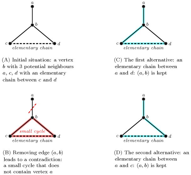
Since all variables of the collection have to take distinct values one can reuse the algorithms associated with the constraint. A second necessary condition is to have no more than one strongly connected component. Pruning for enforcing this condition can be done by forcing all strong bridges to belong to the final solution, since otherwise the strongly connected component would be broken apart. A third necessary condition is that, if the graph is bipartite then the number of vertices of each class should be identical. Consequently if the number of vertices is odd (i.e., is odd) the graph should not be bipartite. Further necessary conditions (useful when the graph is sparse) combining the fact that we have a perfect matching and a single strongly connected component can be found in [ShufetBerliner94]. These conditions forget about the orientation of the arcs of the graph and characterise new required elementary chains. A typical pattern involving four vertices is depicted by Figure 5.66.2 where we assume that:
There is an elementary chain between and (depicted by a dashed edge),
has exactly 3 neighbours.
In this context the edge between and is mandatory in any covering (i.e., the arc from to or the arc from to ) since otherwise a small circuit involving , and would be created.
Figure 5.66.2. Reasoning about elementary chains and degrees: if we have an elementary chain between and and if has 3 neighbours then the edge is mandatory.
When the graph is planar [HopcroftTarjan74][Deo76] one can also use as a necessary condition discovered by Grinberg [Grinberg68] for pruning.
Finally, another approach based an the notion of 1-toughness [Chvatal73] was proposed in [KayaHooker06] and evaluated for small graphs (i.e., graphs with up to 15 vertices).
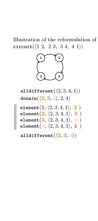
- Reformulation
Let and respectively denotes the number of vertices (i.e., ) and the successor variables associated with vertices . The constraint can be reformulated as a conjunction of one constraint, two constraints, and constraints.
First, we state an constraint for enforcing distinct values to be assigned to the successor variables.
Second, the key idea is, starting from vertex 1, to successively extract the vertices of the circuit until we come back on vertex 1, where (with ) denotes the successor of and the successor of vertex 1. Since we have one single circuit all the should be different from 1. Consequently we state a constraint for declaring their initial domains. To express the link between consecutive we also state a conjunction of constraints of the form:
Finally we add a redundant constraint for stating that all (with ) are distinct, i.e. .
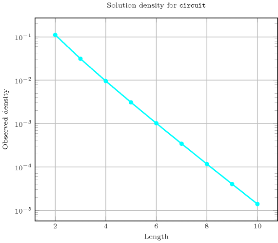
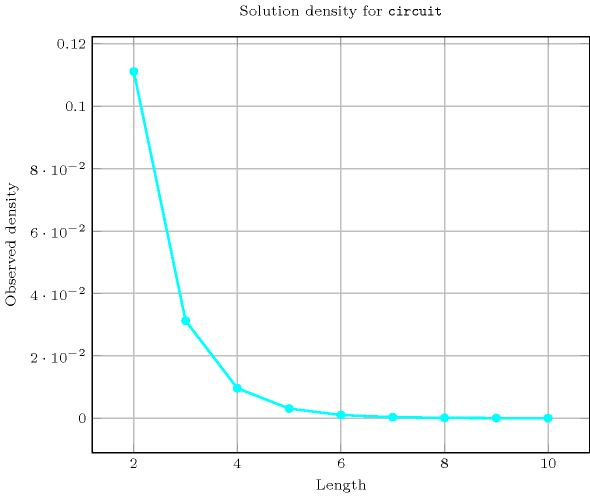
- Counting
-
Length () 2 3 4 5 6 7 8 9 10 Solutions 1 2 6 24 120 720 5040 40320 362880 Number of solutions for : domains
- Systems
- See also
common keyword: (permutation), (graph constraint, one_succ), (graph partitioning constraint, one_succ), (permutation, one_succ), (graph partitioning constraint, Hamiltonian).
generalisation: (introduce a variable for the number of circuits).
implies: , , .
implies (items to collection): .
related: .
- Keywords
combinatorial object: permutation.
constraint type: graph constraint, graph partitioning constraint.
filtering: linear programming, planarity test, strong bridge, DFS-bottleneck.
- Cond. implications
- Arc input(s)
- Arc generator
-
- Arc arity
- Arc constraint(s)
- Graph property(ies)
-
- Graph class
-
- Graph model
The first graph property enforces to have a single strongly connected component containing vertices. The second graph property imposes to only have circuits. Since each vertex of the final graph has only one successor we do not need to use set variables for representing the successors of a vertex.
Parts (A) and (B) of Figure 5.66.3 respectively show the initial and final graph associated with the Example slot. The constraint holds since the final graph consists of one circuit mentioning once every vertex of the initial graph.
Figure 5.66.3. Initial and final graph of the constraint
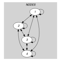
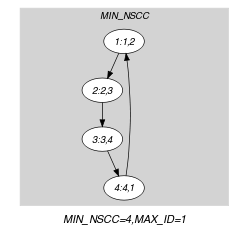
(a) (b)