5.85. connect_points
| DESCRIPTION | LINKS | GRAPH |
- Origin
N. Beldiceanu
- Constraint
- Arguments
- Restrictions
- Purpose
On a 3-dimensional grid of variables, number of groups, where a group consists of a connected set of variables that all have a same value distinct from 0.
- Example
-
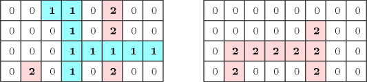
Figure 5.85.1 corresponds to the solution where we describe separately each layer of the grid. The constraint holds since we have two groups (): a first one for the variables of the collection assigned to value 1, and a second one for the variables assigned to value 2.
Figure 5.85.1. The two layers of the solution
- Typical
- Symmetry
All occurrences of two distinct values of that are both different from 0 can be swapped; all occurrences of a value of that is different from 0 can be renamed to any unused value that is also different from 0.
- Arg. properties
Functional dependency: determined by , , and .
- Usage
Wiring problems [Simonis90], [Zhou96].
- Algorithm
Since the graph corresponding to the 3-dimensional grid is symmetric one could certainly use as a starting point the filtering algorithm associated with the number of connected components graph property described in [BeldiceanuPetitRochart06] (see the paragraphs “Estimating ” and “Estimating ”). One may also try to take advantage of the fact that the considered initial graph is a grid in order to simplify the previous filtering algorithm.
- Keywords
characteristic of a constraint: joker value.
final graph structure: strongly connected component, symmetric.
geometry: geometrical constraint.
- Arc input(s)
- Arc generator
-
- Arc arity
- Arc constraint(s)
-
- Graph property(ies)
-
- Graph class
-
- Graph model
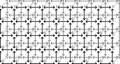
Figure 5.85.2 gives the initial graph constructed by the arc generator associated with the Example slot.
Figure 5.85.2. Graph generated by ([8,4,2])