Global Constraint Catalog: Csame

5.334. same

DESCRIPTION

LINKS

GRAPH

AUTOMATON

Origin

N. Beldiceanu

Constraint

$𝚜𝚊𝚖𝚎 (𝚅𝙰𝚁𝙸𝙰𝙱𝙻𝙴𝚂 1, 𝚅𝙰𝚁𝙸𝙰𝙱𝙻𝙴𝚂 2)$

Arguments

$𝚅𝙰𝚁𝙸𝙰𝙱𝙻𝙴𝚂 1$	$𝚌𝚘𝚕𝚕𝚎𝚌𝚝𝚒𝚘𝚗 (𝚟𝚊𝚛 - 𝚍𝚟𝚊𝚛)$
$𝚅𝙰𝚁𝙸𝙰𝙱𝙻𝙴𝚂 2$	$𝚌𝚘𝚕𝚕𝚎𝚌𝚝𝚒𝚘𝚗 (𝚟𝚊𝚛 - 𝚍𝚟𝚊𝚛)$

Restrictions

| 𝚅𝙰𝚁𝙸𝙰𝙱𝙻𝙴𝚂 1 | = | 𝚅𝙰𝚁𝙸𝙰𝙱𝙻𝙴𝚂 2 |

𝚛𝚎𝚚𝚞𝚒𝚛𝚎𝚍

(𝚅𝙰𝚁𝙸𝙰𝙱𝙻𝙴𝚂 1, 𝚟𝚊𝚛)

𝚛𝚎𝚚𝚞𝚒𝚛𝚎𝚍

(𝚅𝙰𝚁𝙸𝙰𝙱𝙻𝙴𝚂 2, 𝚟𝚊𝚛)

Purpose

The variables of the $𝚅𝙰𝚁𝙸𝙰𝙱𝙻𝙴𝚂 2$ collection correspond to the variables of the $𝚅𝙰𝚁𝙸𝙰𝙱𝙻𝙴𝚂 1$ collection according to a permutation.

Example

(〈1, 9, 1, 5, 2, 1〉, 〈9, 1, 1, 1, 2, 5〉)

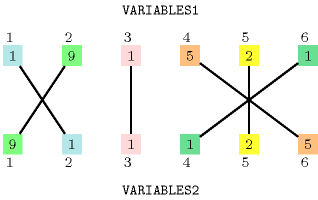
The $𝚜𝚊𝚖𝚎$ constraint holds since values 1, 2, 5 and 9 have the same number of occurrences within both collections $〈 1, 9, 1, 5, 2, 1 〉$ and $〈 9, 1, 1, 1, 2, 5 〉$ . Figure 5.334.1 illustrates this correspondence.

Figure 5.334.1. Illustration of the correspondence between the items of the $𝚅𝙰𝚁𝙸𝙰𝙱𝙻𝙴𝚂 1$ and of the $𝚅𝙰𝚁𝙸𝙰𝙱𝙻𝙴𝚂 2$ collections of the Example slot

All solutions

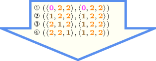
Figure 5.334.2 gives all solutions to the following non ground instance of the $𝚜𝚊𝚖𝚎$ constraint: $U_{1} \in [0, 2]$ , $U_{2} \in [1, 2]$ , $U_{3} \in [1, 2]$ , $V_{1} \in [0, 1]$ , $V_{2} \in [2, 4]$ , $V_{3} \in [2, 3]$ , $𝚜𝚊𝚖𝚎$ $(〈 U_{1}, U_{2}, U_{3} 〉, 〈 V_{1}, V_{2}, V_{3} 〉)$ .

Figure 5.334.2. All solutions corresponding to the non ground example of the $𝚜𝚊𝚖𝚎$ constraint of the All solutions slot where identical values are coloured in the same way in both collections

Typical

| 𝚅𝙰𝚁𝙸𝙰𝙱𝙻𝙴𝚂 1 | > 1

𝚛𝚊𝚗𝚐𝚎

(𝚅𝙰𝚁𝙸𝙰𝙱𝙻𝙴𝚂 1 . 𝚟𝚊𝚛) > 1

𝚛𝚊𝚗𝚐𝚎

(𝚅𝙰𝚁𝙸𝙰𝙱𝙻𝙴𝚂 2 . 𝚟𝚊𝚛) > 1

Symmetries

Arguments are permutable w.r.t. permutation $(𝚅𝙰𝚁𝙸𝙰𝙱𝙻𝙴𝚂 1, 𝚅𝙰𝚁𝙸𝙰𝙱𝙻𝙴𝚂 2)$ .
Items of $𝚅𝙰𝚁𝙸𝙰𝙱𝙻𝙴𝚂 1$ are permutable.
Items of $𝚅𝙰𝚁𝙸𝙰𝙱𝙻𝙴𝚂 2$ are permutable.
All occurrences of two distinct values in $𝚅𝙰𝚁𝙸𝙰𝙱𝙻𝙴𝚂 1 . 𝚟𝚊𝚛$ or $𝚅𝙰𝚁𝙸𝙰𝙱𝙻𝙴𝚂 2 . 𝚟𝚊𝚛$ can be swapped; all occurrences of a value in $𝚅𝙰𝚁𝙸𝙰𝙱𝙻𝙴𝚂 1 . 𝚟𝚊𝚛$ or $𝚅𝙰𝚁𝙸𝙰𝙱𝙻𝙴𝚂 2 . 𝚟𝚊𝚛$ can be renamed to any unused value.

Arg. properties

Aggregate: $𝚅𝙰𝚁𝙸𝙰𝙱𝙻𝙴𝚂 1 (𝚞𝚗𝚒𝚘𝚗)$ , $𝚅𝙰𝚁𝙸𝙰𝙱𝙻𝙴𝚂 2 (𝚞𝚗𝚒𝚘𝚗)$ .

Usage

The $𝚜𝚊𝚖𝚎$ constraint can be used in the following contexts:

Pairing problems taken from [BeldiceanuKatrielThiel04b]. The organisation Doctors Without Borders has a list of doctors and a list of nurses, each of whom volunteered to go on one mission in the next year. Each volunteer specifies a list of possible dates and each mission involves one doctor and one nurse. The task is to produce a list of pairs such that each pair includes a doctor and a nurse who are available at the same date and each volunteer appears in exactly one pair. The problem is modelled by a $𝚜𝚊𝚖𝚎$ $(D = d_{1}, d_{2}, \dots, d_{m}, N = n_{1}, n_{2}, \dots, n_{m})$ constraint where each doctor is represented by a domain variable in $D$ and each nurse by a domain variable in $N$ . For a given doctor or nurse the corresponding domain variable gives the dates when the person is available. When the number of nurses is different from the number of doctors we replace the $𝚜𝚊𝚖𝚎$ constraint by a $𝚞𝚜𝚎𝚍_𝚋𝚢$ constraint.
Timetabling problems where we wish to produce fair schedules for different persons is a second use of the $𝚜𝚊𝚖𝚎$ constraint. Assume we need to generate a plan over a period of $D$ consecutive days for $P$ persons. For each day $d$ and each person $p$ we need to decide whether person $p$ works in the morning shift, in the afternoon shift, in the night shift or does not work at all on day $d$ . In a fair schedule, the number of morning shifts should be the same for all the persons. The same condition holds for the afternoon and the night shifts as well as for the days off. We create for each person $p$ the sequence of variables $v_{p, 1}, v_{p, 2}, \dots, v_{p, D}$ . $v_{p, D}$ is equal to one of $0, 1, 2$ and 3, depending on whether person $p$ does not work, works in the morning, in the afternoon or during the night on day $d$ . We can use $P - 1$ $𝚜𝚊𝚖𝚎$ constraints to express the fact that $v_{1, 1}, v_{1, 2}, \dots, v_{1, D}$ should be a permutation of $v_{p, 1}, v_{p, 2}, \dots, v_{p, D}$ for each $(1 < p \leq P)$ .
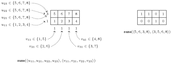
The $𝚜𝚊𝚖𝚎$ constraint can also be used as a channelling constraint for modelling the following recurring pattern: given the number of 1s in each line and each column of a 0-1 matrix $ℳ$ with $n$ rows and $m$ columns, reconstruct the matrix. This pattern usually occurs with additional constraints about compatible positions of the 1s, or about the overall shape reconstructed from all the 1's (e.g., convexity, connectivity). If we restrict ourselves to the basic pattern there is an $O (m n)$ algorithm for reconstructing a $m \cdot n$ matrix from its horizontal and vertical directions [Gale57]. We show how to model this pattern with the $𝚜𝚊𝚖𝚎$ constraint. Let $l_{i}$ $(1 \leq i \leq n)$ and $c_{j}$ $(1 \leq j \leq m)$ denote respectively, the required number of 1s in the $i^{t h}$ row and the $j^{t h}$ column of $ℳ$ . We number the entries of the matrix as shown in the left-hand side of 5.334.3. For row $i$ we create $l_{i}$ domain variables $v_{i k}$ where $k \in [1, l_{i}]$ . Similarly, for each column $j$ we create $c_{j}$ domain variables $u_{j k}$ where $k \in [1, c_{i}]$ . The domain of each variable contains the set of entries that belong to the row or column that the variable corresponds to. Thus, each domain variable represents a 1 that appears in the designated row or column. Let $𝒱$ be the set of variables corresponding to rows and $𝒰$ be the set of variables corresponding to columns. To make sure that each 1 is placed in a different entry, we impose the constraint $𝚊𝚕𝚕𝚍𝚒𝚏𝚏𝚎𝚛𝚎𝚗𝚝$ $(𝒰)$ . In addition, the constraint $𝚜𝚊𝚖𝚎$ $(𝒰, 𝒱)$ enforces that the 1s exactly coincide on the rows and the columns. A solution is shown on the right-hand side of 5.334.3. Note that the $𝚜𝚊𝚖𝚎_𝚊𝚗𝚍_𝚐𝚕𝚘𝚋𝚊𝚕_𝚌𝚊𝚛𝚍𝚒𝚗𝚊𝚕𝚒𝚝𝚢$ constraint allows to model the matrix reconstruction problem without the additional $𝚊𝚕𝚕𝚍𝚒𝚏𝚏𝚎𝚛𝚎𝚗𝚝$ constraint.

Figure 5.334.3. Modelling the 0-1 matrix reconstruction problem with the $𝚜𝚊𝚖𝚎$ constraint (variable $u_{11}$ corresponds to the position of value 1 in the first row, variables $u_{21}$ , $u_{22}$ , $u_{23}$ correspond to the position of value 1 in the second row, and variables $v_{11}$ , $v_{21}$ , $v_{31}$ , $v_{41}$ respectively to the positions of value 1 in the first, second, third and fourth columns)

Remark

The $𝚜𝚊𝚖𝚎$ constraint is a relaxed version of the $𝚜𝚘𝚛𝚝$ constraint introduced in [OlderSwinkelsEmden95]. We do not enforce the second collection of variables to be sorted in increasing order.

If we interpret the collections $𝚅𝙰𝚁𝙸𝙰𝙱𝙻𝙴𝚂 1$ and $𝚅𝙰𝚁𝙸𝙰𝙱𝙻𝙴𝚂 2$ as two multisets variables [KiziltanWalsh02], the $𝚜𝚊𝚖𝚎$ constraint can be considered as an equality constraint between two multisets variables.

The $𝚜𝚊𝚖𝚎$ constraint can be modelled by two $𝚐𝚕𝚘𝚋𝚊𝚕_𝚌𝚊𝚛𝚍𝚒𝚗𝚊𝚕𝚒𝚝𝚢$ constraints. For instance, the $𝚜𝚊𝚖𝚎$ constraint

𝚜𝚊𝚖𝚎 (\begin{matrix} 〈\begin{matrix} 𝚟𝚊𝚛 - x_{1}, 𝚟𝚊𝚛 - x_{2} \end{matrix}〉, \\ 〈\begin{matrix} 𝚟𝚊𝚛 - y_{1}, 𝚟𝚊𝚛 - y_{2} \end{matrix}〉, \end{matrix})

where the union of the domains of the different variables is ${1, 2, 3, 4}$ corresponds to the conjunction of the following two $𝚐𝚕𝚘𝚋𝚊𝚕_𝚌𝚊𝚛𝚍𝚒𝚗𝚊𝚕𝚒𝚝𝚢$ constraints:

𝚐𝚕𝚘𝚋𝚊𝚕_𝚌𝚊𝚛𝚍𝚒𝚗𝚊𝚕𝚒𝚝𝚢 (\begin{matrix} 〈\begin{matrix} 𝚟𝚊𝚛 - x_{1}, 𝚟𝚊𝚛 - x_{2} \end{matrix}〉, \\ 〈\begin{matrix} 𝚟𝚊𝚕 - 1 & 𝚗𝚘𝚌𝚌𝚞𝚛𝚛𝚎𝚗𝚌𝚎 - c_{1}, \\ 𝚟𝚊𝚕 - 2 & 𝚗𝚘𝚌𝚌𝚞𝚛𝚛𝚎𝚗𝚌𝚎 - c_{2}, \\ 𝚟𝚊𝚕 - 3 & 𝚗𝚘𝚌𝚌𝚞𝚛𝚛𝚎𝚗𝚌𝚎 - c_{3}, \\ 𝚟𝚊𝚕 - 4 & 𝚗𝚘𝚌𝚌𝚞𝚛𝚛𝚎𝚗𝚌𝚎 - c_{4} \end{matrix}〉 \end{matrix})

𝚐𝚕𝚘𝚋𝚊𝚕_𝚌𝚊𝚛𝚍𝚒𝚗𝚊𝚕𝚒𝚝𝚢 (\begin{matrix} 〈\begin{matrix} 𝚟𝚊𝚛 - y_{1}, 𝚟𝚊𝚛 - y_{2} \end{matrix}〉, \\ 〈\begin{matrix} 𝚟𝚊𝚕 - 1 & 𝚗𝚘𝚌𝚌𝚞𝚛𝚛𝚎𝚗𝚌𝚎 - c_{1}, \\ 𝚟𝚊𝚕 - 2 & 𝚗𝚘𝚌𝚌𝚞𝚛𝚛𝚎𝚗𝚌𝚎 - c_{2}, \\ 𝚟𝚊𝚕 - 3 & 𝚗𝚘𝚌𝚌𝚞𝚛𝚛𝚎𝚗𝚌𝚎 - c_{3}, \\ 𝚟𝚊𝚕 - 4 & 𝚗𝚘𝚌𝚌𝚞𝚛𝚛𝚎𝚗𝚌𝚎 - c_{4} \end{matrix}〉 \end{matrix})

As shown by the next example, the consistency for all variables of the two $𝚐𝚕𝚘𝚋𝚊𝚕_𝚌𝚊𝚛𝚍𝚒𝚗𝚊𝚕𝚒𝚝𝚢$ constraints does not implies consistency for the corresponding $𝚜𝚊𝚖𝚎$ constraint. This is for instance the case when the domains of $x_{1}$ , $x_{2}$ , $y_{1}$ and $y_{2}$ is respectively equal to ${1, 2}$ , ${3, 4}$ , ${1, 2, 3, 4}$ and ${3, 4}$ . The conjunction of the two $𝚐𝚕𝚘𝚋𝚊𝚕_𝚌𝚊𝚛𝚍𝚒𝚗𝚊𝚕𝚒𝚝𝚢$ constraints does not remove values 3 and 4 from $y_{1}$ .

In his PhD thesis, W.-J. van Hoeve introduces a soft version of the $𝚜𝚊𝚖𝚎$ constraint where the cost is the minimum number of variables to assign differently in order to get back to a solution [vanHoeve05]. In the context of the $𝚜𝚊𝚖𝚎$ constraint this violation cost corresponds to the difference between the number of variables in $𝚅𝙰𝚁𝙸𝙰𝙱𝙻𝙴𝚂 1$ and the number of values that both occur in $𝚅𝙰𝚁𝙸𝙰𝙱𝙻𝙴𝚂 1$ and in $𝚅𝙰𝚁𝙸𝙰𝙱𝙻𝙴𝚂 2$ (provided that one value of $𝚅𝙰𝚁𝙸𝙰𝙱𝙻𝙴𝚂 1$ matches at most one value of $𝚅𝙰𝚁𝙸𝙰𝙱𝙻𝙴𝚂 2$ ).

Algorithm

In [BeldiceanuKatrielThiel04a], [BeldiceanuKatrielThiel04b], [BeldiceanuKatrielThiel05], [Katriel05], it is shown how to model this constraint by a flow network that enables to compute arc-consistency and bound-consistency. The rightmost part of Figure 3.7.30 illustrates this flow model. Unlike the networks used for $𝚊𝚕𝚕𝚍𝚒𝚏𝚏𝚎𝚛𝚎𝚗𝚝$ and $𝚐𝚕𝚘𝚋𝚊𝚕_𝚌𝚊𝚛𝚍𝚒𝚗𝚊𝚕𝚒𝚝𝚢$ , the network now has three sets of nodes, so the algorithms are more complex, in particular the efficient bound-consistency algorithm.

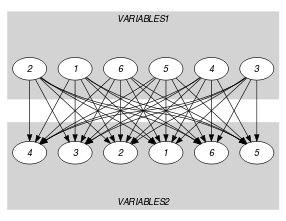
More recently [Cymer12], [CymerPhD13] presents a second filtering algorithm also achieving arc-consistency based on a mapping of the solutions to the $𝚜𝚊𝚖𝚎$ constraint to perfect matchings in a bipartite intersection graph derived from the domain of the variables of the constraint in the following way. To each variable of the $𝚅𝙰𝚁𝙸𝙰𝙱𝙻𝙴𝚂 1$ and $𝚅𝙰𝚁𝙸𝙰𝙱𝙻𝙴𝚂 2$ collection corresponds a vertex of the intersection graph. There is an edge between a vertex associated with a variable of the $𝚅𝙰𝚁𝙸𝙰𝙱𝙻𝙴𝚂 1$ collection and a vertex associated with a variable of the $𝚅𝙰𝚁𝙸𝙰𝙱𝙻𝙴𝚂 2$ collection if and only if the corresponding variables have at least one value in common in their domains.

Reformulation

The $𝚜𝚊𝚖𝚎$ $(𝚅𝙰𝚁𝙸𝙰𝙱𝙻𝙴𝚂 1, 𝚅𝙰𝚁𝙸𝙰𝙱𝙻𝙴𝚂 2)$ constraint can be reformulated as the conjunction $𝚜𝚘𝚛𝚝$ $(𝚅𝙰𝚁𝙸𝙰𝙱𝙻𝙴𝚂 1, 𝚂𝙾𝚁𝚃𝙴𝙳_𝚅𝙰𝚁𝙸𝙰𝙱𝙻𝙴𝚂) \land$ $𝚜𝚘𝚛𝚝$ $(𝚅𝙰𝚁𝙸𝙰𝙱𝙻𝙴𝚂 2, 𝚂𝙾𝚁𝚃𝙴𝙳_𝚅𝙰𝚁𝙸𝙰𝙱𝙻𝙴𝚂)$ .

Used in

$𝚔_𝚜𝚊𝚖𝚎$ .

See also

generalisation: $𝚌𝚘𝚛𝚛𝚎𝚜𝚙𝚘𝚗𝚍𝚎𝚗𝚌𝚎$ ( $𝙿𝙴𝚁𝙼𝚄𝚃𝙰𝚃𝙸𝙾𝙽$ parameter added), $𝚜𝚊𝚖𝚎_𝚒𝚗𝚝𝚎𝚛𝚟𝚊𝚕$ ( $𝚟𝚊𝚛𝚒𝚊𝚋𝚕𝚎$ replaced by $𝚟𝚊𝚛𝚒𝚊𝚋𝚕𝚎 / 𝚌𝚘𝚗𝚜𝚝𝚊𝚗𝚝$ ), $𝚜𝚊𝚖𝚎_𝚖𝚘𝚍𝚞𝚕𝚘$ ( $𝚟𝚊𝚛𝚒𝚊𝚋𝚕𝚎$ replaced by $𝚟𝚊𝚛𝚒𝚊𝚋𝚕𝚎 \mod 𝚌𝚘𝚗𝚜𝚝𝚊𝚗𝚝$ ), $𝚜𝚊𝚖𝚎_𝚙𝚊𝚛𝚝𝚒𝚝𝚒𝚘𝚗$ ( $𝚟𝚊𝚛𝚒𝚊𝚋𝚕𝚎$ replaced by $𝚟𝚊𝚛𝚒𝚊𝚋𝚕𝚎 \in 𝚙𝚊𝚛𝚝𝚒𝚝𝚒𝚘𝚗$ ).

implied by: $𝚕𝚎𝚡_𝚎𝚚𝚞𝚊𝚕$ , $𝚜𝚊𝚖𝚎_𝚊𝚗𝚍_𝚐𝚕𝚘𝚋𝚊𝚕_𝚌𝚊𝚛𝚍𝚒𝚗𝚊𝚕𝚒𝚝𝚢$ , $𝚜𝚊𝚖𝚎_𝚊𝚗𝚍_𝚐𝚕𝚘𝚋𝚊𝚕_𝚌𝚊𝚛𝚍𝚒𝚗𝚊𝚕𝚒𝚝𝚢_𝚕𝚘𝚠_𝚞𝚙$ , $𝚜𝚘𝚛𝚝$ .

implies: $𝚜𝚊𝚖𝚎_𝚒𝚗𝚝𝚎𝚛𝚜𝚎𝚌𝚝𝚒𝚘𝚗$ , $𝚞𝚜𝚎𝚍_𝚋𝚢$ .

soft variant: $𝚜𝚘𝚏𝚝_𝚜𝚊𝚖𝚎_𝚟𝚊𝚛$ (variable-based violation measure).

system of constraints: $𝚔_𝚜𝚊𝚖𝚎$ .

used in reformulation: $𝚜𝚘𝚛𝚝$ .

Keywords

characteristic of a constraint: sort based reformulation, automaton, automaton with array of counters.

combinatorial object: permutation, multiset.

constraint arguments: constraint between two collections of variables.

filtering: bipartite matching, flow, arc-consistency, bound-consistency, DFS-bottleneck.

modelling: channelling constraint, equality between multisets.

Arc input(s)

$𝚅𝙰𝚁𝙸𝙰𝙱𝙻𝙴𝚂 1$ $𝚅𝙰𝚁𝙸𝙰𝙱𝙻𝙴𝚂 2$

Arc generator

𝑃𝑅𝑂𝐷𝑈𝐶𝑇

\mapsto 𝚌𝚘𝚕𝚕𝚎𝚌𝚝𝚒𝚘𝚗 (𝚟𝚊𝚛𝚒𝚊𝚋𝚕𝚎𝚜 1, 𝚟𝚊𝚛𝚒𝚊𝚋𝚕𝚎𝚜 2)

Arc arity

Arc constraint(s)

𝚟𝚊𝚛𝚒𝚊𝚋𝚕𝚎𝚜 1 . 𝚟𝚊𝚛 = 𝚟𝚊𝚛𝚒𝚊𝚋𝚕𝚎𝚜 2 . 𝚟𝚊𝚛

Graph property(ies)

• for all connected components:

𝐍𝐒𝐎𝐔𝐑𝐂𝐄

=

𝐍𝐒𝐈𝐍𝐊

•

𝐍𝐒𝐎𝐔𝐑𝐂𝐄

= | 𝚅𝙰𝚁𝙸𝙰𝙱𝙻𝙴𝚂 1 |

•

𝐍𝐒𝐈𝐍𝐊

= | 𝚅𝙰𝚁𝙸𝙰𝙱𝙻𝙴𝚂 2 |

Graph model

Parts (A) and (B) of Figure 5.334.4 respectively show the initial and final graph associated with the Example slot. Since we use the $𝐍𝐒𝐎𝐔𝐑𝐂𝐄$ and $𝐍𝐒𝐈𝐍𝐊$ graph properties, the source and sink vertices of the final graph are stressed with a double circle. Since there is a constraint on each connected component of the final graph we also show the different connected components. Each of them corresponds to an equivalence class according to the arc constraint. The $𝚜𝚊𝚖𝚎$ constraint holds since:

Each connected component of the final graph has the same number of sources and of sinks.
The number of sources of the final graph is equal to $| 𝚅𝙰𝚁𝙸𝙰𝙱𝙻𝙴𝚂 1 |$ .
The number of sinks of the final graph is equal to $| 𝚅𝙰𝚁𝙸𝙰𝙱𝙻𝙴𝚂 2 |$ .

Figure 5.334.4. Initial and final graph of the $𝚜𝚊𝚖𝚎$ constraint

(a)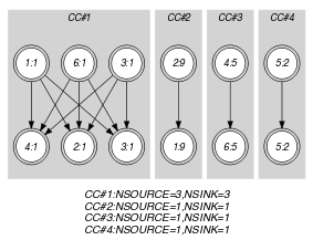

(b)

Signature

Since the initial graph contains only sources and sinks, and since isolated vertices are eliminated from the final graph, we make the following observations:

Sources of the initial graph cannot become sinks of the final graph,
Sinks of the initial graph cannot become sources of the final graph.

From the previous observations and since we use the $𝑃𝑅𝑂𝐷𝑈𝐶𝑇$ arc generator on the collections $𝚅𝙰𝚁𝙸𝙰𝙱𝙻𝙴𝚂 1$ and $𝚅𝙰𝚁𝙸𝙰𝙱𝙻𝙴𝚂 2$ , we have that the maximum number of sources and sinks of the final graph is respectively equal to $| 𝚅𝙰𝚁𝙸𝙰𝙱𝙻𝙴𝚂 1 |$ and $| 𝚅𝙰𝚁𝙸𝙰𝙱𝙻𝙴𝚂 2 |$ . Therefore we can rewrite $𝐍𝐒𝐎𝐔𝐑𝐂𝐄 = | 𝚅𝙰𝚁𝙸𝙰𝙱𝙻𝙴𝚂 1 |$ to $𝐍𝐒𝐎𝐔𝐑𝐂𝐄 \geq | 𝚅𝙰𝚁𝙸𝙰𝙱𝙻𝙴𝚂 1 |$ and simplify $\underset{̲}{\bar{𝐍𝐒𝐎𝐔𝐑𝐂𝐄}}$ to $\bar{𝐍𝐒𝐎𝐔𝐑𝐂𝐄}$ . In a similar way, we can rewrite $𝐍𝐒𝐈𝐍𝐊 = | 𝚅𝙰𝚁𝙸𝙰𝙱𝙻𝙴𝚂 2 |$ to $𝐍𝐒𝐈𝐍𝐊 \geq | 𝚅𝙰𝚁𝙸𝙰𝙱𝙻𝙴𝚂 2 |$ and simplify $\underset{̲}{\bar{𝐍𝐒𝐈𝐍𝐊}}$ to $\bar{𝐍𝐒𝐈𝐍𝐊}$ .

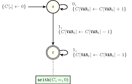
Automaton: To each item of the collection $𝚅𝙰𝚁𝙸𝙰𝙱𝙻𝙴𝚂 1$ corresponds a signature variable $S_{i}$ that is equal to 0. To each item of the collection $𝚅𝙰𝚁𝙸𝙰𝙱𝙻𝙴𝚂 2$ corresponds a signature variable $S_{i + | 𝚅𝙰𝚁𝙸𝙰𝙱𝙻𝙴𝚂 1 |}$ that is equal to 1.

Figure 5.334.5. Automaton of the $𝚜𝚊𝚖𝚎$ constraint

Global Constraint Catalog

5. Global Constraint Catalogue

5.334. same

Figure 5.334.1. Illustration of the correspondence between the items of the $𝚅𝙰𝚁𝙸𝙰𝙱𝙻𝙴𝚂 1$ and of the $𝚅𝙰𝚁𝙸𝙰𝙱𝙻𝙴𝚂 2$ collections of the Example slot

Figure 5.334.2. All solutions corresponding to the non ground example of the $𝚜𝚊𝚖𝚎$ constraint of the All solutions slot where identical values are coloured in the same way in both collections

Figure 5.334.4. Initial and final graph of the $𝚜𝚊𝚖𝚎$ constraint

Figure 5.334.5. Automaton of the $𝚜𝚊𝚖𝚎$ constraint

Global Constraint Catalog

5. Global Constraint Catalogue

5.334. same

Figure 5.334.1. Illustration of the correspondence between the items of the 𝚅𝙰𝚁𝙸𝙰𝙱𝙻𝙴𝚂1 and of the 𝚅𝙰𝚁𝙸𝙰𝙱𝙻𝙴𝚂2 collections of the Example slot

Figure 5.334.2. All solutions corresponding to the non ground example of the 𝚜𝚊𝚖𝚎 constraint of the All solutions slot where identical values are coloured in the same way in both collections

Figure 5.334.4. Initial and final graph of the 𝚜𝚊𝚖𝚎 constraint

Figure 5.334.5. Automaton of the 𝚜𝚊𝚖𝚎 constraint

Figure 5.334.1. Illustration of the correspondence between the items of the $𝚅𝙰𝚁𝙸𝙰𝙱𝙻𝙴𝚂 1$ and of the $𝚅𝙰𝚁𝙸𝙰𝙱𝙻𝙴𝚂 2$ collections of the Example slot

Figure 5.334.2. All solutions corresponding to the non ground example of the $𝚜𝚊𝚖𝚎$ constraint of the All solutions slot where identical values are coloured in the same way in both collections

Figure 5.334.4. Initial and final graph of the $𝚜𝚊𝚖𝚎$ constraint

Figure 5.334.5. Automaton of the $𝚜𝚊𝚖𝚎$ constraint