3.7.79. Degree of diversity of a set of solutions
modelling: degree of diversity of a set of solutions A constraint that allows finding a set of solutions with a certain degree of diversity. As an example, consider the problem of finding 9 diverse solutions for the 10-queens problem. For this purpose we create a 10 by 9 matrix of domain variables taking their values in interval . Each row of corresponds to a solution to the 10-queens problem. We assume that the variables of are assigned row by row, and that within a given row, they are assigned from the first to the last column. Moreover values are tried in increasing order. We first post for each row of the 3 constraints related to the 10-queens problem (see Figure 5.12.2 for an illustration of the 3 constraints). With a constraint, we lexicographically order the first two variables of each row of in order to enforce that the first two variables of any pair of solutions are always distinct. We then impose a constraint on the variables of each column of . Let denote the corresponding cost variable associated with the constraint of the -th column of (i.e., the first argument of the constraint). We put a maximum limit (e.g., 3 in our example) on these cost variables. We also impose that the sum of these cost variables should not exceed a given maximum value (e.g., 8 in our example). Finally, in order to balance the diversity over consecutive variables we state that the sum of two consecutive cost variables should not exceed a given threshold (e.g., 2 in our example). As one of the possible results we get the following nine solutions depicted below.
,
,
,
,
,
,
,
,
.
The costs associated with the constraints of columns are respectively equal to 1, 1, 1, 0, 1, 0, 1, 1, 1, and 1. The different types of constraints between the previous 9 solutions are illustrated by Figure 3.7.23. The nine diverse solutions are shown by Figure 3.7.24. Figure 3.7.25 depicts the distribution of all the queens of the nine solutions on a unique chessboard.
Figure 3.7.23. Constraint network associated with the problem of finding 9 diverse solutions for the 10-queens problem where variables are fixed to the solutions corresponding to , , , , and where each type of constraint (hyperedge) is drawn with its own colour
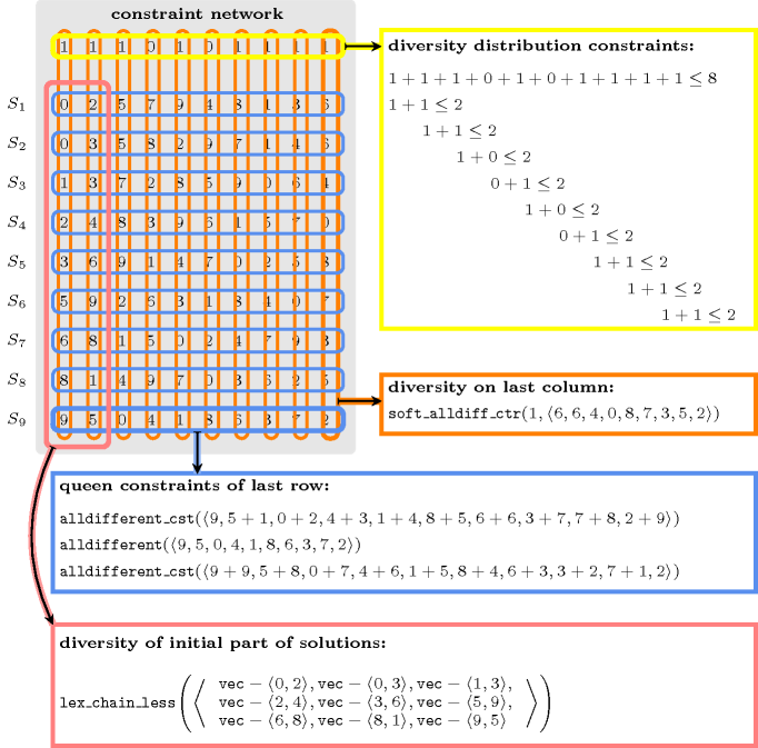
Figure 3.7.24. Nine diverse solutions to the 10-queens problem
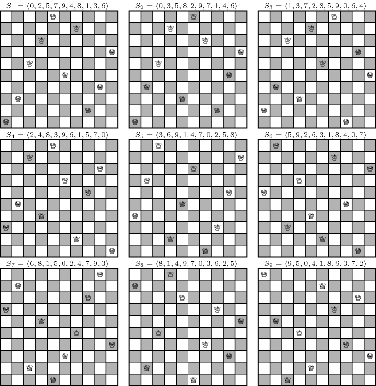
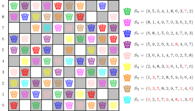
Figure 3.7.25. Distribution of the queens on the chessboard of the nine diverse solutions depicted by Figure 3.7.24 to the 10-queens problem: a red queen means two queens from two different solutions that are placed on a same cell, non-red queens of a same colour are queens that belong to a same solution; out of the cells of the original chessboard, cells are occupied by a single queen, 8 by two queens, and 18 by no queen at all.
Approaches for finding diverse and similar solutions based on the Hamming distances between each pair of solutions are presented by E. Hebrard et al. [HebrardHnichSullivanWalsh05].