2.1.3. Filtering view

Once we know that a constraint for which not all variables are fixed yet is potentially feasible, the next question is to identify variable-value pairs of the form $(\mathrm{𝑣𝑎𝑟},\mathrm{𝑣𝑎𝑙})$ such that, if value $\mathrm{𝑣𝑎𝑙}$ is assigned to variable $\mathrm{𝑣𝑎𝑟}$, the constraint has no solution. Since removing such values reduces a priori the search space, filtering is strongly supported by the implicit motto of constraint programming that the more you prune the better. Assuming that you already have a necessary and sufficient condition that can be evaluated in polynomial time for checking whether a constraint has at least one solution or not, you can directly reuse it for checking whether a value can be assigned or not to a variable. Since the number of variable-value pairs to check may be quadratic with respect to the total number of variables and values one usually prefers developing a dedicated filtering algorithm that is less costly than checking the feasibility condition on each variable-value pair.

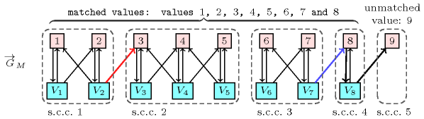
For the $\mathrm{𝚊𝚕𝚕𝚍𝚒𝚏𝚏𝚎𝚛𝚎𝚗𝚝}$ constraint a first filtering algorithm [Regin94] is based on a characterisation of the edges of the variable-value graph that belong to a maximum matching but not to all. A matching on a graph is a set of edges of the graph such that no two edges have a vertex in common; it is maximum if its number of edges is maximum. We first introduce a digraph ${\overrightarrow{G}}_M$ that is associated with a matching $M$ that matches all variables of the $\mathrm{𝚊𝚕𝚕𝚍𝚒𝚏𝚏𝚎𝚛𝚎𝚗𝚝}$ constraint. The vertices of ${\overrightarrow{G}}_M$ are defined as the variables and the values that can be assigned to the variables of the $\mathrm{𝚊𝚕𝚕𝚍𝚒𝚏𝚏𝚎𝚛𝚎𝚗𝚝}$ constraint. To each value $\mathrm{𝑣𝑎𝑙}$ that can be assigned to a variable $\mathrm{𝑣𝑎𝑟}$ corresponds an arc of ${\overrightarrow{G}}_M$ from $\mathrm{𝑣𝑎𝑟}$ to $\mathrm{𝑣𝑎𝑙}$. Finally, if value $\mathrm{𝑣𝑎𝑙}$ is matched to variable $\mathrm{𝑣𝑎𝑟}$ in the matching $M$ we add the reverse arc from $\mathrm{𝑣𝑎𝑙}$ to $\mathrm{𝑣𝑎𝑟}$ to the arcs of ${\overrightarrow{G}}_M$. Now a variable $\mathrm{𝑣𝑎𝑟}$ can be assigned a value $\mathrm{𝑣𝑎𝑙}$ if and only if $\mathrm{𝑣𝑎𝑟}$ and $\mathrm{𝑣𝑎𝑙}$ belong to the same strongly connected component of ${\overrightarrow{G}}_M$ or if there is a path consisting of distinct vertices and arcs of ${\overrightarrow{G}}_M$ that start with $(\mathrm{𝑣𝑎𝑟},\mathrm{𝑣𝑎𝑙})$ and ends up in an unmatched value with respect to matching $M$, see [Thiel04].

Figure 2.1.1. Illustration of the filtering for $\mathrm{𝚊𝚕𝚕𝚍𝚒𝚏𝚏𝚎𝚛𝚎𝚗𝚝}$$\left(\langle V_1,V_2,V_3,V_4,V_5,V_6,V_7,V_8\rangle \right)$ with $V_1\in [1,2]$, $V_2\in [1,3]$, $V_3\in [3,4]$, $V_4\in [3,5]$, $V_5\in [4,5]$, $V_6\in [6,7]$, $V_7\in [6,8]$, $V_8\in [8,9]$ with respect to the maximum matching $M$ defined by $V_i=i$ ($1\le i\le 8$) and the corresponding digraph and its five strongly connected components s.c.c. $k$ ($1\le k\le 5$): 8 can be assigned to $V_7$ (blue arc) since the path $\left(V_{7}8V_{8}9\right)$ ends up in an unmatched value, but 3 cannot be assigned to $V_2$ (red arc) since 3 and $V_2$ do not belong to the same strongly connected component and since there is no path from $V_2$ to the unique unmatched value 9.

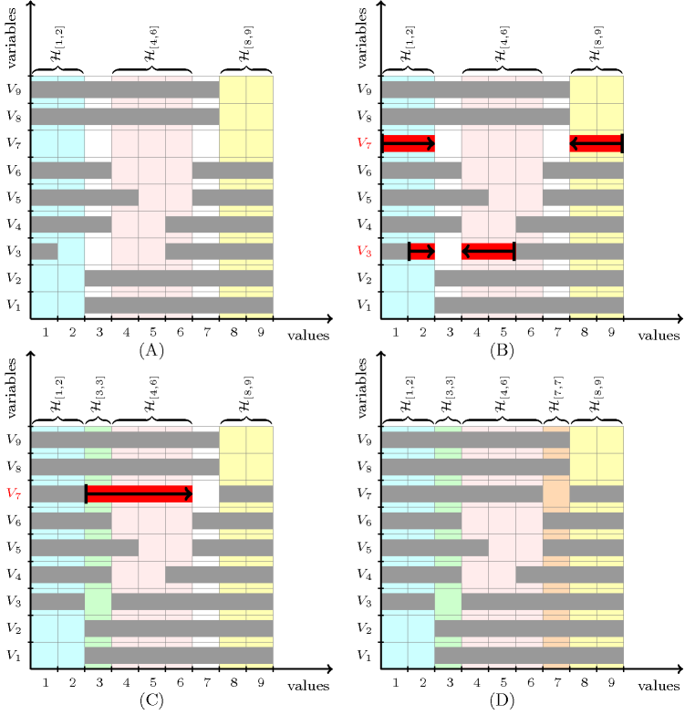
Another filtering algorithm for $\mathrm{𝚊𝚕𝚕𝚍𝚒𝚏𝚏𝚎𝚛𝚎𝚗𝚝}$ based on Hall intervals just focuses on adjusting the minimum and maximum values of the variables. Given a set of domain variables, a Hall interval is an interval of values $[\mathrm{𝑙𝑜𝑤},\mathrm{𝑢𝑝}]$ denoted by ${\mathscr{H}}_{[\mathrm{𝑙𝑜𝑤},\mathrm{𝑢𝑝}]}$ such that there are $\mathrm{𝑢𝑝}-\mathrm{𝑙𝑜𝑤}+1$ variables whose domains are contained in ${\mathscr{H}}_{[\mathrm{𝑙𝑜𝑤},\mathrm{𝑢𝑝}]}$. A minimal Hall interval ${\mathscr{H}}_{[\mathrm{𝑙𝑜𝑤},\mathrm{𝑢𝑝}]}$ is a Hall interval that does not contain any Hall interval ${\mathscr{H}}_{[{\mathrm{𝑙𝑜𝑤}}^{\text{'}},{\mathrm{𝑢𝑝}}^{\text{'}}]}$ such that either $\mathrm{𝑙𝑜𝑤}={\mathrm{𝑙𝑜𝑤}}^{\text{'}}$ or $\mathrm{𝑢𝑝}={\mathrm{𝑢𝑝}}^{\text{'}}$. Given a Hall interval $\mathscr{H}$ and a variable $V$ whose domain is not included in $\mathscr{H}$ but intersects $\mathscr{H}$, the idea is to adjust the minimum (respectively maximum) value of variable $V$ to the smallest (respectively largest) value that does not belong to $\mathscr{H}$. Figure 2.1.2 illustrates this idea on the constraint $\mathrm{𝚊𝚕𝚕𝚍𝚒𝚏𝚏𝚎𝚛𝚎𝚗𝚝}$$\left(\langle V_1,V_2,V_3,V_4,V_5,V_6,V_7,V_8,V_9\rangle \right)$ with $V_1\in [1,2]$, $V_2\in [1,2]$, $V_3\in [2,5]$, $V_4\in [4,5]$, $V_5\in [5,6]$, $V_6\in [4,6]$, $V_7\in [1,9]$, $V_8\in [8,9]$, $V_9\in [8,9]$.

• Part (A) of Figure 2.1.2 shows in light blue, in light pink and in light yellow the three minimal Hall intervals associated with the initial domains of variables $V_1,V_2,\cdots ,V_9$.

  • ${\mathscr{H}}_{[1,2]}$ corresponds to interval $[1,2]$, which contains the domains of $V_1$ and $V_2$.

  • ${\mathscr{H}}_{[4,6]}$ corresponds to interval $[4,6]$, which contains the domains of $V_4$, $V_5$ and $V_6$.

  • ${\mathscr{H}}_{[8,9]}$ corresponds to interval $[8,9]$, which contains the domains of $V_8$ and $V_9$.

• Part (B) of Figure 2.1.2 shows the first propagation step with respect to the Hall intervals ${\mathscr{H}}_{[1,2]}$, ${\mathscr{H}}_{[4,6]}$ and ${\mathscr{H}}_{[8,9]}$. First note that variables $V_3$ and $V_7$ are the only variables whose domain is not included in a Hall interval. Consequently $V_3$ and $V_7$ are candidates for adjusting their minimum or maximum domain values.

  • Since the minimum value of $V_3$, that is i.e. value 2, belongs to the Hall interval ${\mathscr{H}}_{[1,2]}$ we adjust the minimum of $V_3$ to the smallest value that does not yet belong to any Hall interval, i.e. value 3.

  • Since the maximum value of $V_3$, that is i.e. value 5, belongs to the Hall interval ${\mathscr{H}}_{[4,6]}$ we adjust the maximum value of $V_3$ to the largest value that does not yet belong to any Hall interval, i.e. value 3.

  • Since the minimum value of $V_7$, that is i.e. value 1, belongs to the Hall interval ${\mathscr{H}}_{[1,2]}$ we adjust the minimum of $V_7$ to the smallest value that does not yet belong to any Hall interval, i.e. value 3.

  • Since the maximum value of $V_7$, that is i.e. value 9, belongs to the Hall interval ${\mathscr{H}}_{[8,9]}$ we adjust the maximum of $V_7$ to the largest value that does not yet belong to any Hall interval, that is i.e. value 7.

• Part (C) of Figure 2.1.2 shows the second propagation step with respect to the new Hall interval ${\mathscr{H}}_{[3,3]}$. Now $V_7$ is the only variable whose domain is not included in a Hall interval so it is a candidate for adjusting its minimum or maximum domain value.

  • Since the minimum value of $V_7$, i.e. value 3, belongs to the new Hall interval ${\mathscr{H}}_{[3,3]}$ we adjust the minimum of $V_7$ to the smallest value that does not yet belong to any Hall interval, i.e. value 7.

• Finally, part (D) of Figure 2.1.2 shows all the minimal Hall intervals after reaching the fix point of the filtering, where ${\mathscr{H}}_{[7,7]}$ is a new minimal Hall interval.

Figure 2.1.2. Steps (A), (B), (C) and (D) for filtering the minimum and maximum values wrt Hall intervals ${\mathscr{H}}_{[\mathrm{𝑙𝑜𝑤},\mathrm{𝑢𝑝}]}$ for $\mathrm{𝚊𝚕𝚕𝚍𝚒𝚏𝚏𝚎𝚛𝚎𝚗𝚝}$$\left(\langle V_1,V_2,V_3,V_4,V_5,V_6,V_7,V_8,V_9\rangle \right)$ with $V_1\in [1,2]$, $V_2\in [1,2]$, $V_3\in [2,5]$, $V_4\in [4,5]$, $V_5\in [5,6]$, $V_6\in [4,6]$, $V_7\in [1,9]$, $V_8\in [8,9]$, $V_9\in [8,9]$. Each horizontal grey strip corresponds to a set of consecutive values that do not belong to the domain of a variable, while each horizontal red strip represents an adjustment of the minimum or the maximum value of the domain of a variable.