3.7.153. Minimum cost flow
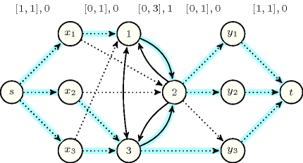
A constraint for which there is a filtering algorithm based on an algorithm that finds a minimum cost flow in a graph. This graph is usually constructed from the variables of the constraint as well as from their potential values. Figure 3.7.42 illustrates the minimum cost flow model used for the constraint. The demand and the capacity of the arcs are depicted by an interval on top of the corresponding arcs. The weight is given after that interval: a weight of 0 (respectively 1) is depicted by a dotted (respectively plain) arc. Weights of 1 are assigned to arcs linking two values since they model the correction of a discrepancy between variables , , and variables , , . Blue arcs represent the feasible flow corresponding to the solution .
Figure 3.7.42. Minimum cost flow model for the constraint described in Table 3.7.42
| 1 | 1 | ||
| 2 | 2 | ||
| 3 | 3 |