• $\mathrm{𝚊𝚕𝚕𝚍𝚒𝚏𝚏𝚎𝚛𝚎𝚗𝚝}$,

• $\mathrm{𝚊𝚖𝚘𝚗𝚐}\_\mathrm{𝚜𝚎𝚚}$,

• $\mathrm{𝚐𝚕𝚘𝚋𝚊𝚕}\_\mathrm{𝚌𝚊𝚛𝚍𝚒𝚗𝚊𝚕𝚒𝚝𝚢}$,

• $\mathrm{𝚐𝚕𝚘𝚋𝚊𝚕}\_\mathrm{𝚌𝚊𝚛𝚍𝚒𝚗𝚊𝚕𝚒𝚝𝚢}\_\mathrm{𝚕𝚘𝚠}\_\mathrm{𝚞𝚙}$,

• $\mathrm{𝚐𝚕𝚘𝚋𝚊𝚕}\_\mathrm{𝚌𝚊𝚛𝚍𝚒𝚗𝚊𝚕𝚒𝚝𝚢}\_\mathrm{𝚕𝚘𝚠}\_\mathrm{𝚞𝚙}\_\mathrm{𝚗𝚘}\_\mathrm{𝚕𝚘𝚘𝚙}$,

• $\mathrm{𝚐𝚕𝚘𝚋𝚊𝚕}\_\mathrm{𝚌𝚊𝚛𝚍𝚒𝚗𝚊𝚕𝚒𝚝𝚢}\_\mathrm{𝚗𝚘}\_\mathrm{𝚕𝚘𝚘𝚙}$,

• $\mathrm{𝚘𝚙𝚎𝚗}\_\mathrm{𝚊𝚕𝚕𝚍𝚒𝚏𝚏𝚎𝚛𝚎𝚗𝚝}$,

• $\mathrm{𝚘𝚙𝚎𝚗}\_\mathrm{𝚐𝚕𝚘𝚋𝚊𝚕}\_\mathrm{𝚌𝚊𝚛𝚍𝚒𝚗𝚊𝚕𝚒𝚝𝚢}$,

• $\mathrm{𝚘𝚙𝚎𝚗}\_\mathrm{𝚐𝚕𝚘𝚋𝚊𝚕}\_\mathrm{𝚌𝚊𝚛𝚍𝚒𝚗𝚊𝚕𝚒𝚝𝚢}\_\mathrm{𝚕𝚘𝚠}\_\mathrm{𝚞𝚙}$,

• $\mathrm{𝚜𝚊𝚖𝚎}$,

• $\mathrm{𝚜𝚊𝚖𝚎}\_\mathrm{𝚊𝚗𝚍}\_\mathrm{𝚐𝚕𝚘𝚋𝚊𝚕}\_\mathrm{𝚌𝚊𝚛𝚍𝚒𝚗𝚊𝚕𝚒𝚝𝚢}$,

• $\mathrm{𝚜𝚊𝚖𝚎}\_\mathrm{𝚊𝚗𝚍}\_\mathrm{𝚐𝚕𝚘𝚋𝚊𝚕}\_\mathrm{𝚌𝚊𝚛𝚍𝚒𝚗𝚊𝚕𝚒𝚝𝚢}\_\mathrm{𝚕𝚘𝚠}\_\mathrm{𝚞𝚙}$,

• $\mathrm{𝚜𝚕𝚒𝚍𝚒𝚗𝚐}\_\mathrm{𝚜𝚞𝚖}$,

• $\mathrm{𝚜𝚢𝚖𝚖𝚎𝚝𝚛𝚒𝚌}\_\mathrm{𝚌𝚊𝚛𝚍𝚒𝚗𝚊𝚕𝚒𝚝𝚢}$,

• $\mathrm{𝚜𝚢𝚖𝚖𝚎𝚝𝚛𝚒𝚌}\_\mathrm{𝚐𝚌𝚌}$,

• $\mathrm{𝚞𝚜𝚎𝚍}\_\mathrm{𝚋𝚢}$.

A constraint for which there is a filtering algorithm based on an algorithm that finds a feasible flow in a graph. The graph is usually constructedSometimes it is also constructed from the reformulation of a global constraint in term of a conjunction of linear constraints. This is for instance the case for the $\mathrm{𝚊𝚖𝚘𝚗𝚐}\_\mathrm{𝚜𝚎𝚚}$ and the $\mathrm{𝚜𝚕𝚒𝚍𝚒𝚗𝚐}\_\mathrm{𝚜𝚞𝚖}$ global constraints. from the variables of the constraint as well as from their potential values. The usual game is to come up with a flow model such that there exists a one to one correspondence between feasible flows in the flow model and solutions to the constraint, so that detecting arcs that cannot carry any flow in any feasible flow will lead removing some values from the domains of some variables. The next sections provide standard flow models for the $\mathrm{𝚊𝚕𝚕𝚍𝚒𝚏𝚏𝚎𝚛𝚎𝚗𝚝}$, the $\mathrm{𝚘𝚙𝚎𝚗}\_\mathrm{𝚊𝚕𝚕𝚍𝚒𝚏𝚏𝚎𝚛𝚎𝚗𝚝}$, the $\mathrm{𝚐𝚕𝚘𝚋𝚊𝚕}\_\mathrm{𝚌𝚊𝚛𝚍𝚒𝚗𝚊𝚕𝚒𝚝𝚢}\_\mathrm{𝚕𝚘𝚠}\_\mathrm{𝚞𝚙}$, the $\mathrm{𝚐𝚕𝚘𝚋𝚊𝚕}\_\mathrm{𝚌𝚊𝚛𝚍𝚒𝚗𝚊𝚕𝚒𝚝𝚢}\_\mathrm{𝚕𝚘𝚠}\_\mathrm{𝚞𝚙}\_\mathrm{𝚗𝚘}\_\mathrm{𝚕𝚘𝚘𝚙}$, the $\mathrm{𝚞𝚜𝚎𝚍}\_\mathrm{𝚋𝚢}$, the $\mathrm{𝚜𝚊𝚖𝚎}$, and the $\mathrm{𝚜𝚊𝚖𝚎}\_\mathrm{𝚊𝚗𝚍}\_\mathrm{𝚐𝚕𝚘𝚋𝚊𝚕}\_\mathrm{𝚌𝚊𝚛𝚍𝚒𝚗𝚊𝚕𝚒𝚝𝚢}\_\mathrm{𝚕𝚘𝚠}\_\mathrm{𝚞𝚙}$ constraints.

A. Flow models for the $\mathrm{𝚊𝚕𝚕𝚍𝚒𝚏𝚏𝚎𝚛𝚎𝚗𝚝}$ and the $\mathrm{𝚘𝚙𝚎𝚗}\_\mathrm{𝚊𝚕𝚕𝚍𝚒𝚏𝚏𝚎𝚛𝚎𝚗𝚝}$ constraints

Figure 3.7.28 presents flow models for the $\mathrm{𝚊𝚕𝚕𝚍𝚒𝚏𝚏𝚎𝚛𝚎𝚗𝚝}$ and the $\mathrm{𝚘𝚙𝚎𝚗}\_\mathrm{𝚊𝚕𝚕𝚍𝚒𝚏𝚏𝚎𝚛𝚎𝚗𝚝}$ constraints. Blue arcs represent feasible flows respectively corresponding to the solutions $\mathrm{𝚊𝚕𝚕𝚍𝚒𝚏𝚏𝚎𝚛𝚎𝚗𝚝}$$\left(\langle x_1=1,x_2=2,x_3=3,x_4=4,x_5=5\rangle \right)$ and $\mathrm{𝚘𝚙𝚎𝚗}\_\mathrm{𝚊𝚕𝚕𝚍𝚒𝚏𝚏𝚎𝚛𝚎𝚗𝚝}$$(\{\mathbf{1},\mathbf{2},\mathbf{3},\mathbf{5}\},\langle x_1=1,x_2=2,x_3=3,x_4=3,x_5=4\rangle )$, while red arcs correspond to arcs that cannot carry any flow if the constraint has a solution. Tables 3.7.27 and 3.7.27 respectively provide the initial domains of the variables we assume for the $\mathrm{𝚊𝚕𝚕𝚍𝚒𝚏𝚏𝚎𝚛𝚎𝚗𝚝}$ and $\mathrm{𝚘𝚙𝚎𝚗}\_\mathrm{𝚊𝚕𝚕𝚍𝚒𝚏𝚏𝚎𝚛𝚎𝚗𝚝}$ constraints.

Figure 3.7.28. Flow models for the $\mathrm{𝚊𝚕𝚕𝚍𝚒𝚏𝚏𝚎𝚛𝚎𝚗𝚝}$ and the $\mathrm{𝚘𝚙𝚎𝚗}\_\mathrm{𝚊𝚕𝚕𝚍𝚒𝚏𝚏𝚎𝚛𝚎𝚗𝚝}$ constraints described in Tables 3.7.27 and 3.7.27: in both cases a first layer consists of the variables of the constraint and a second layer corresponds to the values that can be assigned to the variables; each arc has a lower and upper capacity regarding the flow it can carry; all variables $x_i$ (with $i\in [1,5]$) such that the minimum capacity of the arc from $s$ to $x_i$ is equal to 1 must be assigned distinct values.

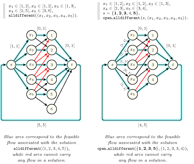
• Within the context of the $\mathrm{𝚊𝚕𝚕𝚍𝚒𝚏𝚏𝚎𝚛𝚎𝚗𝚝}$ constraint the assignments $x_3=1$, $x_3=2$ and $x_4=2$ are forbidden since values 1 and 2 must already be assigned to variables $x_1$ and $x_2$. Finally the assignments $x_4=3$ and $x_5=3$ are also forbidden since values 1, 2 and 3 must be assigned to variables $x_1$, $x_2$ and $x_3$.

• Within the context of the $\mathrm{𝚘𝚙𝚎𝚗}\_\mathrm{𝚊𝚕𝚕𝚍𝚒𝚏𝚏𝚎𝚛𝚎𝚗𝚝}$ constraint, the assignment $x_4=3$ does not matter at all since the position of $x_4$ within $\langle x_1=1,x_2=2,x_3=3,x_4=3,x_5=4\rangle$ (i.e., position 4) does not belong to the set of variables positions $\{1,2,3,5\}$. We can only prune according to those variables that for sure should be assigned distinct values. Consequently $x_3=1$ and $x_3=2$ are forbidden since values 1 and 2 must already be assigned to $x_1$ and $x_2$. Finally the assignment $x_5=3$ is also forbidden since values 1, 2 and 3 must be assigned to $x_1$, $x_2$ and $x_3$.

B. Flow models for the $\mathrm{𝚐𝚕𝚘𝚋𝚊𝚕}\_\mathrm{𝚌𝚊𝚛𝚍𝚒𝚗𝚊𝚕𝚒𝚝𝚢}\_\mathrm{𝚕𝚘𝚠}\_\mathrm{𝚞𝚙}$ and the $\mathrm{𝚐𝚕𝚘𝚋𝚊𝚕}\_\mathrm{𝚌𝚊𝚛𝚍𝚒𝚗𝚊𝚕𝚒𝚝𝚢}\_\mathrm{𝚕𝚘𝚠}\_\mathrm{𝚞𝚙}\_\mathrm{𝚗𝚘}\_\mathrm{𝚕𝚘𝚘𝚙}$ constraints

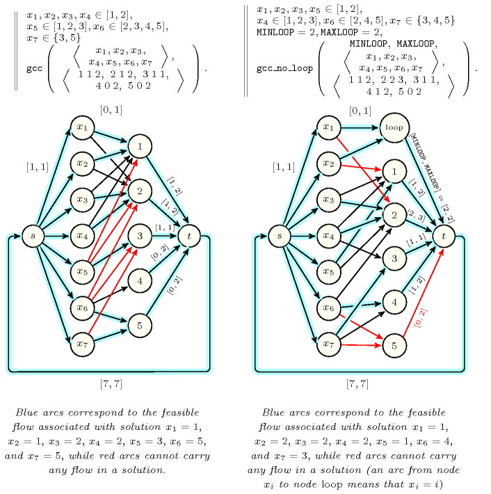
Figure 3.7.29. Flow models for the $\mathrm{𝚐𝚕𝚘𝚋𝚊𝚕}\_\mathrm{𝚌𝚊𝚛𝚍𝚒𝚗𝚊𝚕𝚒𝚝𝚢}\_\mathrm{𝚕𝚘𝚠}\_\mathrm{𝚞𝚙}$ and the $\mathrm{𝚐𝚕𝚘𝚋𝚊𝚕}\_\mathrm{𝚌𝚊𝚛𝚍𝚒𝚗𝚊𝚕𝚒𝚝𝚢}\_\mathrm{𝚕𝚘𝚠}\_\mathrm{𝚞𝚙}\_\mathrm{𝚗𝚘}\_\mathrm{𝚕𝚘𝚘𝚙}$ constraints described in Tables 3.7.29 and 3.7.29: in both cases a first layer consists of the variables of the constraint and a second layer corresponds to the values that can be assigned to the variables (in the second model, the loop node represents an anonymous value $i$ corresponding to assignments of the form $x_i=i$); each arc has a lower and upper capacity regarding the flow it can carry; arcs entering a node associated with a variable must carry a flow of 1 since each variable must be assigned a single value, while arcs exiting a node associated with a value have a capacity set accordingly the last argument of the constraint (i.e., the collection of values $\mathrm{𝚅𝙰𝙻𝚄𝙴𝚂}$).

Figure 3.7.29 presents flow models for the $\mathrm{𝚐𝚕𝚘𝚋𝚊𝚕}\_\mathrm{𝚌𝚊𝚛𝚍𝚒𝚗𝚊𝚕𝚒𝚝𝚢}\_\mathrm{𝚕𝚘𝚠}\_\mathrm{𝚞𝚙}$ and the $\mathrm{𝚐𝚕𝚘𝚋𝚊𝚕}\_\mathrm{𝚌𝚊𝚛𝚍𝚒𝚗𝚊𝚕𝚒𝚝𝚢}\_\mathrm{𝚕𝚘𝚠}\_\mathrm{𝚞𝚙}\_\mathrm{𝚗𝚘}\_\mathrm{𝚕𝚘𝚘𝚙}$ constraints. Blue arcs represent feasible flows respectively corresponding to the solutions $\mathrm{𝚐𝚕𝚘𝚋𝚊𝚕}\_\mathrm{𝚌𝚊𝚛𝚍𝚒𝚗𝚊𝚕𝚒𝚝𝚢}\_\mathrm{𝚕𝚘𝚠}\_\mathrm{𝚞𝚙}$ $(\langle x_1=1,x_2=1,x_3=2,x_4=2,x_5=3,x_6=5,x_7=5\rangle ,\langle \mathrm{𝚟𝚊𝚕}-1\mathrm{𝚘𝚖𝚒𝚗}-1\mathrm{𝚘𝚖𝚊𝚡}-2,\mathrm{𝚟𝚊𝚕}-2\mathrm{𝚘𝚖𝚒𝚗}-1\mathrm{𝚘𝚖𝚊𝚡}-2,\mathrm{𝚟𝚊𝚕}-3\mathrm{𝚘𝚖𝚒𝚗}-1\mathrm{𝚘𝚖𝚊𝚡}-1,\mathrm{𝚟𝚊𝚕}-4\mathrm{𝚘𝚖𝚒𝚗}-0\mathrm{𝚘𝚖𝚊𝚡}-2,\mathrm{𝚟𝚊𝚕}-5\mathrm{𝚘𝚖𝚒𝚗}-0\mathrm{𝚘𝚖𝚊𝚡}-2\rangle )$ and $\mathrm{𝚐𝚕𝚘𝚋𝚊𝚕}\_\mathrm{𝚌𝚊𝚛𝚍𝚒𝚗𝚊𝚕𝚒𝚝𝚢}\_\mathrm{𝚕𝚘𝚠}\_\mathrm{𝚞𝚙}\_\mathrm{𝚗𝚘}\_\mathrm{𝚕𝚘𝚘𝚙}$ $(2,2,\langle x_1=1,x_2=2,x_3=2,x_4=2,x_5=1,x_6=4,x_7=3\rangle ,\langle \mathrm{𝚟𝚊𝚕}-1\mathrm{𝚘𝚖𝚒𝚗}-1\mathrm{𝚘𝚖𝚊𝚡}-2,\mathrm{𝚟𝚊𝚕}-2\mathrm{𝚘𝚖𝚒𝚗}-2\mathrm{𝚘𝚖𝚊𝚡}-3,\mathrm{𝚟𝚊𝚕}-3\mathrm{𝚘𝚖𝚒𝚗}-1\mathrm{𝚘𝚖𝚊𝚡}-1,\mathrm{𝚟𝚊𝚕}-4\mathrm{𝚘𝚖𝚒𝚗}-1\mathrm{𝚘𝚖𝚊𝚡}-2,\mathrm{𝚟𝚊𝚕}-5\mathrm{𝚘𝚖𝚒𝚗}-0\mathrm{𝚘𝚖𝚊𝚡}-2\rangle )$, while red arcs correspond to arcs that cannot carry any flow if the constraint has a solution:

• Within the context of the $\mathrm{𝚐𝚕𝚘𝚋𝚊𝚕}\_\mathrm{𝚌𝚊𝚛𝚍𝚒𝚗𝚊𝚕𝚒𝚝𝚢}\_\mathrm{𝚕𝚘𝚠}\_\mathrm{𝚞𝚙}$ constraint variables $x_1$, $x_2$, $x_3$ and $x_4$ take their values within the set $\{1,2\}$. Since each value in $\{1,2\}$ can be used at most 2 times, variables different from $x_1$, $x_2$, $x_3$, $x_4$ cannot be assigned a value in $\{1,2\}$. Consequently, $x_5\ne 1$, $x_5\ne 2$ and $x_6\ne 2$. Since value 3 is the only remaining value for variable $x_5$, and since value 3 can be assigned to at most one variable, the assignments $x_6\ne 3$ and $x_7\ne 3$ are also forbidden.

• • On the one hand we should have exactly two assignments of the form $x_i=i$ ($i\in [1,7]$), since the first and second arguments of the constraint $\mathrm{𝚐𝚕𝚘𝚋𝚊𝚕}\_\mathrm{𝚌𝚊𝚛𝚍𝚒𝚗𝚊𝚕𝚒𝚝𝚢}\_\mathrm{𝚕𝚘𝚠}\_\mathrm{𝚞𝚙}\_\mathrm{𝚗𝚘}\_\mathrm{𝚕𝚘𝚘𝚙}$ are both set to two. Since the two variables $x_1$ and $x_2$ are the only variables such that $i\in \mathrm{𝑑𝑜𝑚}\left(x_i\right)$ we must have $x_1=1$ and $x_2=2$, i.e. $x_1\ne 2$ and $x_2\ne 1$.

  • On the other hand, since we should have at least $1+2+1+1=5$ assignments of the form $x_i=j$ ($i\ne j,j\in [1,4]$) and since only 5 variables $x_i$ (with $i\in [3,7]$) can be assigned a value $j$ in $[1,4]$ with $i\ne j$, these variables should not be assigned a value outside interval $[1,4]$, i.e. $x_6\ne 5$ and $x_7\ne 5$.

C. Flow models for the $\mathrm{𝚞𝚜𝚎𝚍}\_\mathrm{𝚋𝚢}$ and the $\mathrm{𝚜𝚊𝚖𝚎}$ constraints

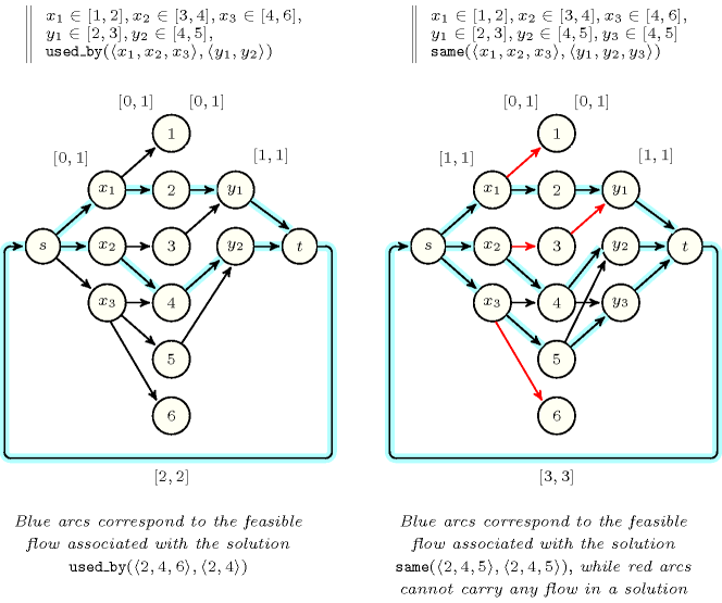
Figure 3.7.30 presents flow models for the $\mathrm{𝚞𝚜𝚎𝚍}\_\mathrm{𝚋𝚢}$ and the $\mathrm{𝚜𝚊𝚖𝚎}$ constraints. Blue arcs represent feasible flows respectively corresponding to the solutions $\mathrm{𝚞𝚜𝚎𝚍}\_\mathrm{𝚋𝚢}$$(\langle x_1=2,x_2=4,x_3=6\rangle ,\langle y_1=2,y_2=4\rangle )$ and $\mathrm{𝚜𝚊𝚖𝚎}$$(\langle x_1=2,x_2=4,x_3=5\rangle ,\langle y_1=2,y_2=4,y_3=5\rangle )$, while red arcs correspond to arcs that cannot carry any flow if the constraint has a solution. Within the context of the $\mathrm{𝚜𝚊𝚖𝚎}$ constraint, the assignment $x_1=1$ is forbidden since $1\notin \mathrm{𝑑𝑜𝑚}\left(y_1\right)\cup \mathrm{𝑑𝑜𝑚}\left(y_2\right)\cup \mathrm{𝑑𝑜𝑚}\left(y_3\right)$. Consequently $x_1=2$ and, since $y_1$ is the only variable of $\{y_1,y_2,y_3\}$ that can be assigned value 2, the assignment $y_1=3$ is forbidden. Now since $3\notin \mathrm{𝑑𝑜𝑚}\left(y_1\right)\cup \mathrm{𝑑𝑜𝑚}\left(y_2\right)\cup \mathrm{𝑑𝑜𝑚}\left(y_3\right)$ the assignment $x_2=3$ is also forbidden. Finally $x_3=6$ is forbidden since $6\notin \mathrm{𝑑𝑜𝑚}\left(y_1\right)\cup \mathrm{𝑑𝑜𝑚}\left(y_2\right)\cup \mathrm{𝑑𝑜𝑚}\left(y_3\right)$.

Figure 3.7.30. Flow models for the $\mathrm{𝚞𝚜𝚎𝚍}\_\mathrm{𝚋𝚢}$ and the $\mathrm{𝚜𝚊𝚖𝚎}$ constraints described in Tables 3.7.30 and 3.7.30: in both cases a first layer consists of the variables $x_i$ of the first argument of both constraints, a second layer corresponds to the values that can be assigned to the variables $x_i$ and $y_i$ (i.e., the first and second arguments), and a third layer consists of the variables $y_i$ of the second argument of both constraints; there is an arc from a variable $x_i$ (resp. $y_i$) to a value $v$ if, and only if, value $v$ can be assigned to variable $x_i$ (resp. $y_i$); each arc has a lower and upper capacity regarding the flow it can carry; since for both constraints each value assigned to a variable of the second argument must also correspond to a value assigned to a variable of the first argument the arcs exiting the $y_i$ must carry a flow of 1.

D. Flow model for the $\mathrm{𝚜𝚊𝚖𝚎}\_\mathrm{𝚊𝚗𝚍}\_\mathrm{𝚐𝚕𝚘𝚋𝚊𝚕}\_\mathrm{𝚌𝚊𝚛𝚍𝚒𝚗𝚊𝚕𝚒𝚝𝚢}\_\mathrm{𝚕𝚘𝚠}\_\mathrm{𝚞𝚙}$ constraint

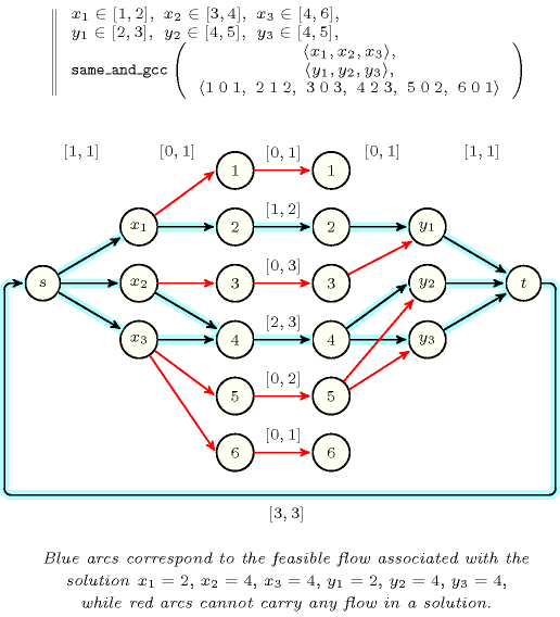
Figure 3.7.31 presents a flow model for the $\mathrm{𝚜𝚊𝚖𝚎}\_\mathrm{𝚊𝚗𝚍}\_\mathrm{𝚐𝚕𝚘𝚋𝚊𝚕}\_\mathrm{𝚌𝚊𝚛𝚍𝚒𝚗𝚊𝚕𝚒𝚝𝚢}\_\mathrm{𝚕𝚘𝚠}\_\mathrm{𝚞𝚙}$ constraint. Blue arcs represent the feasible flow corresponding to the solution $\mathrm{𝚜𝚊𝚖𝚎}\_\mathrm{𝚊𝚗𝚍}\_\mathrm{𝚐𝚕𝚘𝚋𝚊𝚕}\_\mathrm{𝚌𝚊𝚛𝚍𝚒𝚗𝚊𝚕𝚒𝚝𝚢}\_\mathrm{𝚕𝚘𝚠}\_\mathrm{𝚞𝚙}$ $(\langle x_1=2,x_2=4,x_3=4\rangle ,\langle y_1=2,y_2=4,y_3=4\rangle ,\langle \mathrm{𝚟𝚊𝚕}-1\mathrm{𝚘𝚖𝚒𝚗}-0\mathrm{𝚘𝚖𝚊𝚡}-1,\mathrm{𝚟𝚊𝚕}-2\mathrm{𝚘𝚖𝚒𝚗}-1\mathrm{𝚘𝚖𝚊𝚡}-2,\mathrm{𝚟𝚊𝚕}-3\mathrm{𝚘𝚖𝚒𝚗}-0\mathrm{𝚘𝚖𝚊𝚡}-3,\mathrm{𝚟𝚊𝚕}-4\mathrm{𝚘𝚖𝚒𝚗}-2\mathrm{𝚘𝚖𝚊𝚡}-3,\mathrm{𝚟𝚊𝚕}-5\mathrm{𝚘𝚖𝚒𝚗}-0\mathrm{𝚘𝚖𝚊𝚡}-2,\mathrm{𝚟𝚊𝚕}-6\mathrm{𝚘𝚖𝚒𝚗}-0\mathrm{𝚘𝚖𝚊𝚡}-1\rangle )$, while red arcs correspond to arcs that cannot carry any flow if the constraint has a solution. The assignment $x_1=1$ is forbidden since $1\notin \mathrm{𝑑𝑜𝑚}\left(y_1\right)\cup \mathrm{𝑑𝑜𝑚}\left(y_2\right)\cup \mathrm{𝑑𝑜𝑚}\left(y_3\right)$. Consequently $x_1=2$ and, since $y_1$ is the only variable of $\{y_1,y_2,y_3\}$ that can be assigned value 2, the assignment $y_1=3$ is forbidden. Now since $3\notin \mathrm{𝑑𝑜𝑚}\left(y_1\right)\cup \mathrm{𝑑𝑜𝑚}\left(y_2\right)\cup \mathrm{𝑑𝑜𝑚}\left(y_3\right)$ the assignment $x_2=3$ is also forbidden. The assignment $x_3=6$ is forbidden since $6\notin \mathrm{𝑑𝑜𝑚}\left(y_1\right)\cup \mathrm{𝑑𝑜𝑚}\left(y_2\right)\cup \mathrm{𝑑𝑜𝑚}\left(y_3\right)$. Finally $x_3=5$, $y_2=5$ and $y_3=5$ are also forbidden since value 4 must be assigned to at least two variables.

Figure 3.7.31. Flow model for the $\mathrm{𝚜𝚊𝚖𝚎}\_\mathrm{𝚊𝚗𝚍}\_\mathrm{𝚐𝚕𝚘𝚋𝚊𝚕}\_\mathrm{𝚌𝚊𝚛𝚍𝚒𝚗𝚊𝚕𝚒𝚝𝚢}\_\mathrm{𝚕𝚘𝚠}\_\mathrm{𝚞𝚙}$ constraint described in Table 3.7.30: in both cases a first layer consists of the variables $x_i$ of the first argument of the constraint, a second (resp. third) layer corresponds to the values that can be assigned to the variables $x_i$ (resp. $y_i$), and a fourth layer consists of the variables $y_i$ of the second argument of the constraint; each arc has a lower and upper capacity regarding the flow it can carry; values are duplicated in two layers in order to model the minimum and maximum number of occurrences of each value; there is an arc from a variable $x_i$ (resp. $y_i$) to a value $v$ if, and only if, value $v$ can be assigned to variable $x_i$ (resp. $y_i$); since each variable $x_i$ (resp. $y_i$) must be assigned a value the arcs exiting $s$ (resp. entering $t$) must carry a flow of 1.