5.167. global_cardinality_with_costs
| DESCRIPTION | LINKS | GRAPH |
- Origin
- Constraint
- Synonyms
, .
- Arguments
- Restrictions
- Purpose
Each value should be taken by exactly variables of the collection. In addition the of an assignment is equal to the sum of the elementary costs associated with the fact that we assign variable of the collection to the value of the collection. These elementary costs are given by the collection.
- Example
-
The constraint holds since:
Values 3, 5 and 6 respectively occur 3, 0 and 1 times within the collection .
The argument corresponds to the sum of the costs respectively associated with the first, second, third and fourth items of , namely 4, 1, 3 and 6.
- All solutions
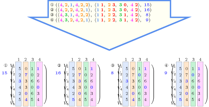
Figure 5.167.1 gives all solutions to the following non ground instance of the constraint:
, , , , , ,
, , , ,
,
,
,
,
,
,
,
,
.
Figure 5.167.1. All solutions corresponding to the non ground example of the constraint of the All solutions slot
- Typical
- Arg. properties
Functional dependency: determined by .
Functional dependency: determined by , and .
- Usage
A classical utilisation of the constraint corresponds to the following assignment problem. We have a set of persons as well as a set of jobs to perform. Each job requires a number of persons restricted to a specified interval. In addition each person has to be assigned to one specific job taken from a subset of . There is a cost associated with the fact that person is assigned to job . The previous problem is modelled with a single constraint where the persons and the jobs respectively correspond to the items of the and collection.
The constraint can also be used for modelling a conjunction and . For this purpose we set the domain of the variables to and the cost attribute of a variable and one of its potential value to . In practice this can be used for the magic squares and the magic hexagon problems where all the are set to 1.
- Algorithm
A filtering algorithm achieving arc-consistency independently on each side (i.e., the greater than or equal to side and the less than or equal to side) of the constraint is described in [Regin99a], [Regin02]. This algorithm assumes for each value a fixed minimum and maximum number of occurrences. If we rather have occurrence variables, the Reformulation slot explains how to also obtain some propagation from the cost variable back to the occurrence variables.
- Reformulation
Let and respectively denote the number of items of the and of the collections. Let denote the values . In addition let (with ) denote the values , i.e., line of the matrix .
By introducing auxiliary variables and , the constraint can be expressed in term of the conjunction of one constraint, constraints and one arithmetic constraint .
For each variable (with ) of the collection a first constraint provides the correspondence between the variable and the index of the value to which it is assigned. A second links the previous index to the cost variable associated with variable . Finally the total cost is equal to the sum .
In the context of the Example slot we get the following conjunction of constraints:
,
.
We now show how to add implied constraints that can also propagate from the cost variable back to the occurrence variables. Let respectively denote the variables . The idea is to get for each value (with ) an idea of its minimum and maximum contribution in the total cost that is linked to the number of times it is assigned to a variables of . E.g., if value (with ) is used twice, then the corresponding minimum (respectively maximum) contribution in the total cost will be at least equal to the sum of the two smallest (respectively largest) costs attached to row . Let (with ) denotes the contribution that stems from the variables of that are assigned value . For each value (with ) we create one constraint for linking to the corresponding minimum contribution . The table of that constraint has entries, where entry (with ) corresponds to the sum of the smallest entries of row of the cost matrix . Similarly we create for each value (with ) one constraint for linking to the corresponding maximum contribution . The table of that constraint also has entries, where entry (with ) corresponds to the sum of the largest entries of row of the cost matrix .
In the context of the cost matrix of the Example slot we get the following conjunction of implied constraints:
,
,
,
,
,
, ,
, ,
, .
- Systems
- See also
attached to cost variant: ( associated with each , pair removed).
common keyword: (cost filtering constraint,weighted assignment), , (weighted assignment).
implies: .
- Keywords
-
constraint arguments: pure functional dependency.
filtering: cost filtering constraint.
heuristics: regret based heuristics, regret based heuristics in matrix problems.
modelling: cost matrix, scalar product, functional dependency.
For all items of :
- Arc input(s)
- Arc generator
-
- Arc arity
- Arc constraint(s)
- Graph property(ies)
-
- Arc input(s)
- Arc generator
-
- Arc arity
- Arc constraint(s)
- Graph property(ies)
-
- Graph model
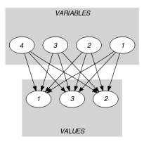
The first graph constraint forces each value of the collection to be taken by a specific number of variables of the collection. It is identical to the graph constraint used in the constraint. The second graph constraint expresses that the variable is equal to the sum of the elementary costs associated with each variable-value assignment. All these elementary costs are recorded in the collection. More precisely, the cost is recorded in the attribute of the entry of the collection. This is ensured by the restriction that enforces the fact that the items of the collection are sorted in lexicographically increasing order according to attributes and .
Parts (A) and (B) of Figure 5.167.2 respectively show the initial and final graph associated with the second graph constraint of the Example slot.
Figure 5.167.2. Initial and final graph of the constraint
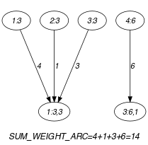
(a) (b)