5.12. alldifferent
| DESCRIPTION | LINKS | GRAPH | AUTOMATON |
- Origin
- Constraint
- Synonyms
, , , , , , .
- Argument
- Restriction
- Purpose
Enforce all variables of the collection to take distinct values.
- Example
-
The constraint holds since all the values 5, 1, 9 and 3 are distinct.
- All solutions
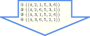
Figure 5.12.1 gives all solutions to the following non ground instance of the constraint: , , , , , , .
Figure 5.12.1. All solutions corresponding to the non ground example of the constraint of the All solutions slot
- Typical
- Symmetries
Items of are permutable.
Two distinct values of can be swapped; a value of can be renamed to any unused value.
- Arg. properties
Contractible wrt. .
- Usage
The constraint occurs in most practical problems directly or indirectly. A classical example is the n-queens chess puzzle problem: Place queens on an by chessboard in such a way that no queen attacks another. Two queens attack each other if they are located on the same column, on the same row, or on the same diagonal. This can be modelled as the conjunction of three constraints. We associate to column of the chessboard a domain variable that gives the row number where the corresponding queen is located. The three constraints are:
for the descending diagonals,
for the rows,
for the ascending diagonals.
They are respectively depicted by parts (A), (C) and (D) of Figure 5.12.2. Figure 5.12.3 makes explicit the link between the two families of diagonals and the corresponding constraints. Note that this model matches the checker introduced by Gauss to test whether a permutation of row numbers is a solution or not to the 8 queens problem: first add the numbers 1 up to 8 to the permutation and check that the resulting numbers are distinct, second add the numbers 8 down to 1 and perform the same check [Watkins04].
Figure 5.12.2. Descending diagonals (A-B), rows (C) and ascending diagonals (D-E)
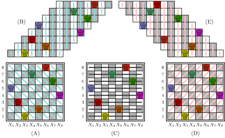
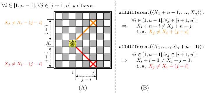
Figure 5.12.3. (A) For every pair of columns , (), given the position of the queen on column , we respectively have from the ascending and descending diagonals that and (B) Equivalence of the two constraints respectively associated with the ascending and descending diagonals with the two families of disequalities (i.e., the orange and the red one) depicted in Part (A)
A second example taken from [AsratianDenleyHaggkvist98], where the bipartite graph associated with the constraint is convex, is a ski assignment problem: “a set of skiers have each specified the smallest and largest ski sizes they will accept from a given set of ski sizes”. The task is to find a ski size for each skier.
Examples such as Costas arrays and Golomb rulers involve one or several constraints on differences of variables.
Quite often, the constraint is also used in conjunction with several constraints, especially in the context of assignment problems [Hooker07book], or with several precedence constraints, especially in the context of symmetry breaking or scheduling problems [BessiereNarodytskaQuimperWalsh11].
Other examples involving several constraints sharing some variables can be found in the Usage slot of the constraint.
- Remark
Even if the constraint did not have this form, it was specified in ALICE [Lauriere76], [Lauriere78] by asking for an injective correspondence between variables and values: . From an algorithmic point of view, the algorithm for computing the cardinality of the maximum matching of a bipartite graph was not used in ALICE for checking the feasibility of the constraint, even though the algorithm was already known in 1976. This is because the goal of ALICE was to show that a general system could be as efficient as dedicated algorithms. For this reason the concluding part of [Lauriere76] explicitly mentions that specialised algorithms should be discarded. On the one hand, many people, especially from the OR community, have complained about such a radical statement [Roy06]. On the other hand, the motivation of such a statement stands from the fact that a truly intelligent system should not rely on black-box algorithms, but should rather be able to reconstruct them from some kind of first principles. How to achieve this is still an open question.
Some solvers use, in a pre-processing phase before stating all constraints, an algorithm for automatically extracting large cliques [BronKerbosch73], [EppsteinStrash11] from a set of binary disequalities in order to replace them by constraints.
W.-J. van Hoeve provides a survey about the constraint in [Hoeve01].
For possible relaxation of the constraints see the , the (i.e., ), the , the and the constraints, and Figure 2.1.4 of Section 2.1.5.
Within the context of linear programming, relaxations of the constraint are described in [WilliamsYan01] and in [Hooker07book].
Within the context of constraint-centered search heuristics, G. Pesant and A. Zanarini [ZanariniPesant07b] have proposed several estimators for evaluating the number of solutions of an constraint (since counting the total number of maximum matchings of the corresponding variable-value graph is #P-complete [Valiant79]). Faster, but less accurate estimators, based on upper bounds of the number of solutions were proposed three years later by the same authors [ZanariniPesant10].
Given variables taking their values within the interval , the total number of solutions to the corresponding constraint corresponds to the sequence A000142 of the On-Line Encyclopaedia of Integer Sequences [Sloane10].
- Algorithm
The first complete filtering algorithm was independently found by M.-C. Costa [Costa94] and J.-C. Régin [Regin94]. This algorithm is based on a corollary of C. Berge that characterises the edges of a graph that belong to a maximum matching but not to all [Berge70].A similar result is in fact given in [Petersen1891]. Similarly, Dulmage-Mendelsohn decomposition [DulmageMendelsohn58] was also used recently by [Cymer12], [CymerPhD13] to characterise such edges and prune the corresponding variables both for the constraint and for other constraints like , , , , , , , , . Assuming that all variables have no holes in their domain, M. Leconte came up with a filtering algorithm [Leconte96] based on edge finding. A first bound-consistency algorithm was proposed by Bleuzen-Guernalec et al. [GuernalecColmerauer97]. Later on, two different approaches were used to design bound-consistency algorithms. Both approaches model the constraint as a bipartite graph. The first identifies Hall intervals in this graph [Puget98], [LopezOrtizQuimperTrompBeek03] and the second applies the same algorithm that is used to compute arc-consistency, but achieves a speedup by exploiting the simpler structure [Glover67] of the graph [MehlhornThiel00]. Ian P. Gent et al. discuss in [GentMiguelNightingale08] implementations issues behind the complete filtering algorithm and in particular the computation of the strongly connected components of the residual graph (i.e., a graph constructed from a maximum variable-value matching and from the possible values of the variables of the constraint), which appears to be the main bottleneck in practice. Figures 2.1.1 and 2.1.2 of Section 2.1.3 illustrate the filtering of the constraint with respect to arc-consistency and bound-consistency. The leftmost part of Figure 3.7.28 illustrates a flow model for the constraint where there is a one-to-one correspondence between feasible flows in the flow model and solutions of the constraint.
From a worst case complexity point of view, assuming that is the number of variables and the sum of the domains sizes, we have the following complexity results:
Complete filtering is achieved in by Régin's algorithm [Regin94].
Range consistency is done in by Leconte's algorithm [Leconte96].
Bound-consistency is performed in in [Puget98], [MehlhornThiel00], [LopezOrtizQuimperTrompBeek03]. If sort can be achieved in linear time, typically when the constraint encodes a permutation,In this context the total number of values that can be assigned to the variables of the constraint is equal to the number of variables. Under this assumption sorting the variables on their minimum or maximum values can be achieved in linear time. the worst case complexity of the algorithms described in [MehlhornThiel00], [LopezOrtizQuimperTrompBeek03] goes down to .
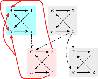
Within the context of explanations [JussienBarichard00], the explanation of the filtering algorithm that achieves arc-consistency for the constraint is described in [Rochart05]. Given the residual graph (i.e., a graph constructed from a maximum variable-value matching and from the possible values of the variables of the constraint), the removal of an arc starting from a vertex belonging to a strongly connected component to a distinct strongly connected component is explained by all missing arcs starting from a descendant component of and ending in an ancestor component of (i.e., since the addition of any of these missing arcs would merge the strongly connected components and ). Let us illustrate this on a concrete example. For this purpose assume we have the following variables and the values that can potentially be assigned to each of them, , , , , , , , . Figure 5.12.4 represents the residual graph associated with the maximum matching corresponding to the assignment , , , , , , , . It has four strongly connected components containing respectively vertices , , and . Arcs that are between strongly connected components correspond to values that can be removed:
The removal of value 2 from variable is explained by the absence of the arcs corresponding to the assignments , , and (since adding any of these missing arcs would merge the blue and the pink strongly connected components containing the vertices corresponding to value 2 and variable ).
The removal of value 6 from variable is explained by the absence of the arcs corresponding to the assignments , , and . Again adding the corresponding arcs would merge the two strongly connected components containing the vertices corresponding to value 6 and variable .
The removal of value 6 from variable is explained by the absence of the arcs corresponding to the assignments , , and .
The removal of value 6 from variable is explained by the absence of the arcs corresponding to the assignments , , and .
Figure 5.12.4. Strongly connected components of the residual graph illustrating the explanation of the removal of a value for the constraint , , , , , , , , : the explanation why value 2 is removed from variable corresponds to all missing arcs whose addition would merge the blue and the pink strongly connected components (i.e., the missing arcs corresponding to the assignments , , and that are depicted by thick pink lines)
An additional example for illustrating the generation of explanations for the constraint when there are more values than variables is provided by Figure 2.1.3 of Section 2.1.4.
After applying bound-consistency the following property holds for all variables of an constraint. Given a Hall interval , any variable whose range intersects without being included in has its minimum value (respectively maximum value ) that is located before (respectively after) the Hall interval (i.e., ).
The constraint is entailed if and only if there is no value that can be assigned two distinct variables of the collection (i.e., the intersection of the two sets of potential values of any pair of variables is empty).
- Reformulation
The constraint can be reformulated into a set of disequalities constraints. This model neither preserves bound-consistency nor arc-consistency:
On the one hand a model, involving linear constraints, preserving bound-consistency was introduced in [BessiereKatsirelosNarodytskaQuimperWalsh09IJCAI]. For each potential interval of consecutive values this model uses 0-1 variables for modelling that each variable of the collection is assigned a value within interval (i.e., ),How to encode the reified constraint with linear constraints is described in the Reformulation slot of the constraint. and an inequality constraint for enforcing the condition that the sum of the corresponding 0-1 variables is less than or equal to the size of the corresponding interval (i.e. ).
On the other hand, it was shown in [BessiereKatsirelosNarodytskaWalsh09] that there is no polynomial sized decomposition that preserves arc-consistency.
Finally the constraint can also be reformulated as the conjunction . Unlike the naive reformulation, i.e., a constraint between each pair of variables, the -based reformulation is linear in space.
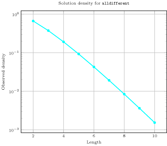
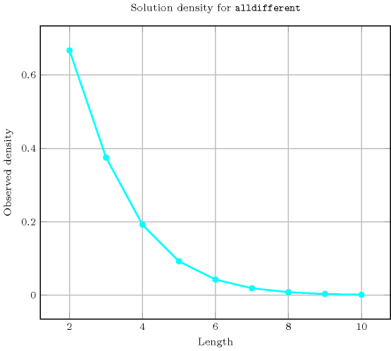
- Counting
-
Length () 2 3 4 5 6 7 8 9 10 Solutions 6 24 120 720 5040 40320 362880 3628800 39916800 Number of solutions for : domains
- Systems
allDifferent in Choco, linear in Gecode, alldifferent in JaCoP, alldiff in JaCoP, alldistinct in JaCoP, all_different in MiniZinc, all_different in SICStus, all_distinct in SICStus.
- Used in
- See also
common keyword: , , , (permutation), (all different), (permutation), , (all different,disequality), (permutation).
cost variant: , .
generalisation: ( replaced by , all of the same size), ( replaced by ), ( replaced by ), ( replaced by ), ( replaced by ), ( replaced by ), ( replaced by orthotope), ( replaced by ), (control the number of occurrence of each value with a counter variable), (control the number of occurrence of each value with an interval), ( replaced by ), (count number of distinct values).
implied by: , , , , .
implies: , , .
part of system of constraints: .
soft variant: (value 0 can be used several times), (open constraint), (decomposition-based violation measure), (variable-based violation measure).
used in reformulation: (bound-consistency preserving reformulation), , .
- Keywords
characteristic of a constraint: core, all different, disequality, sort based reformulation, automaton, automaton with array of counters.
combinatorial object: permutation.
constraint type: system of constraints, value constraint.
filtering: bipartite matching, bipartite matching in convex bipartite graphs, convex bipartite graph, flow, Hall interval, arc-consistency, bound-consistency, SAT, DFS-bottleneck, entailment.
final graph structure: one_succ.
modelling exercises: n-Amazons, zebra puzzle.
problems: maximum clique, graph colouring.
puzzles: n-Amazons, n-queens, Costas arrays, Euler knight, Golomb ruler, magic hexagon, magic square, zebra puzzle, Sudoku.
- Cond. implications
- Arc input(s)
- Arc generator
-
- Arc arity
- Arc constraint(s)
- Graph property(ies)
-
- Graph class
-
- Graph model
We generate a clique with an equality constraint between each pair of vertices (including a vertex and itself) and state that the size of the largest strongly connected component should not exceed one.
Parts (A) and (B) of Figure 5.12.5 respectively show the initial and final graph associated with the Example slot. Since we use the graph property we show one of the largest strongly connected component of the final graph. The holds since all the strongly connected components have at most one vertex: a value is used at most once.
Figure 5.12.5. Initial and final graph of the constraint
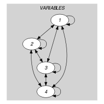
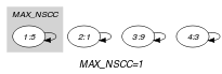
(a) (b)
- Automaton
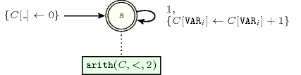
Figure 5.12.6 depicts the automaton associated with the constraint. To each item of the collection corresponds a signature variable that is equal to 1. The automaton counts the number of occurrences of each value and finally imposes that each value is taken at most one time.
Figure 5.12.6. Automaton of the constraint
- Quiz
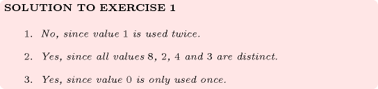
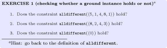
: checking whether a ground instance holds or not
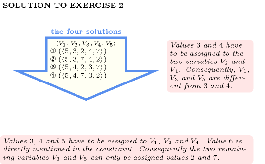
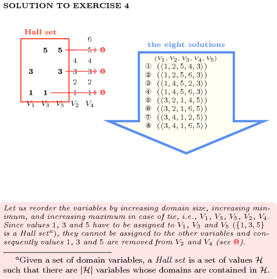
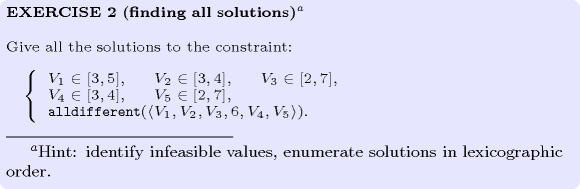
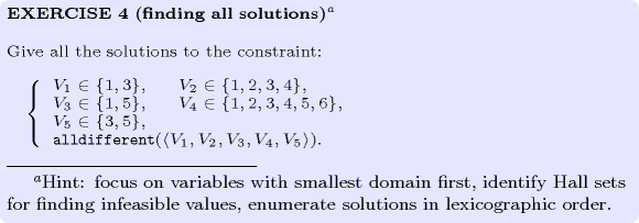
: finding all solutions
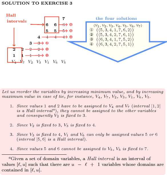
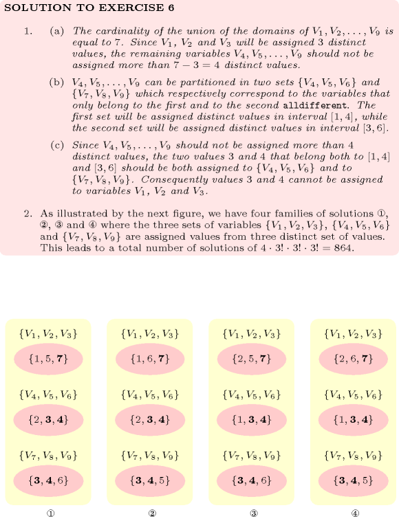
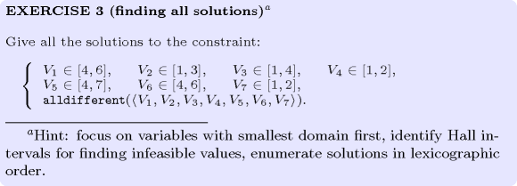
: finding all solutions
: finding all solutions
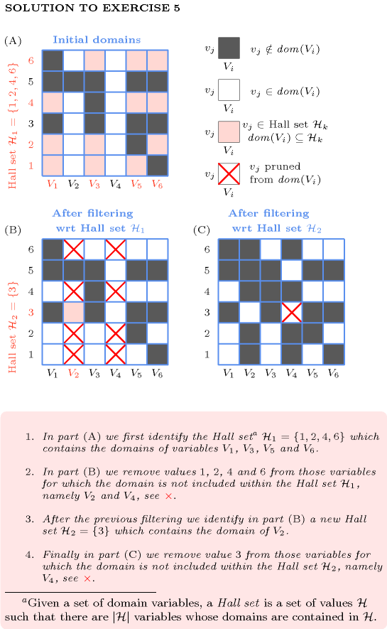
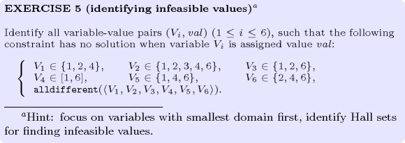
: identifying infeasible values
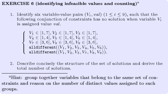
: identifying infeasible values and counting
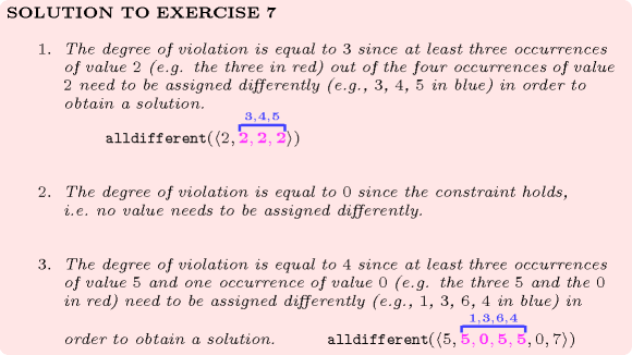
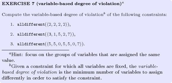
: variable-based degree of violation
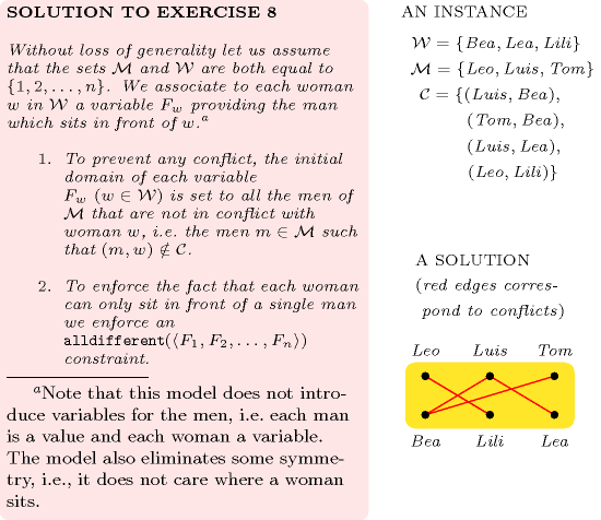
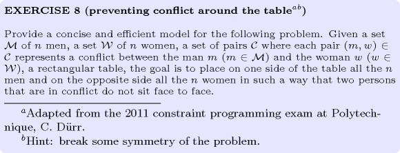
: preventing conflict around the table
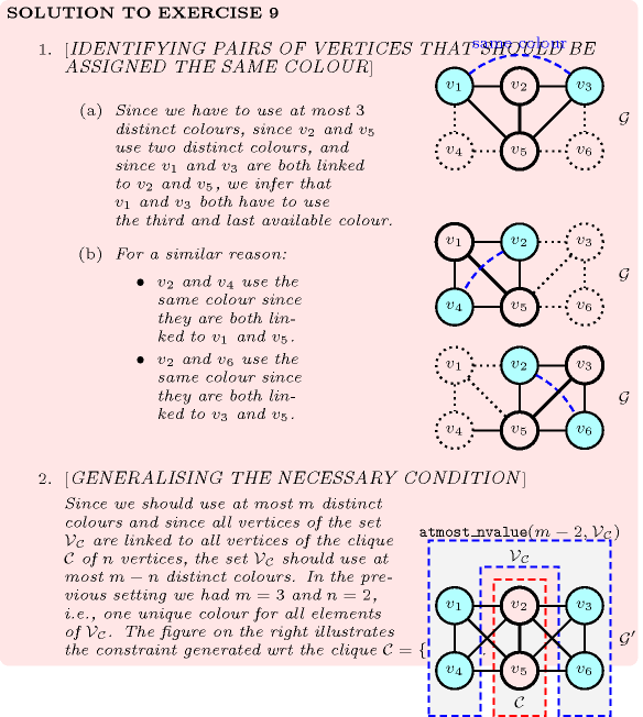
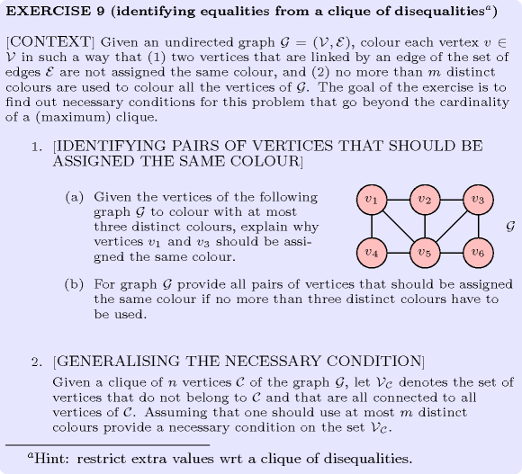
: identifying equalities from a clique of disequalities
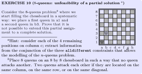
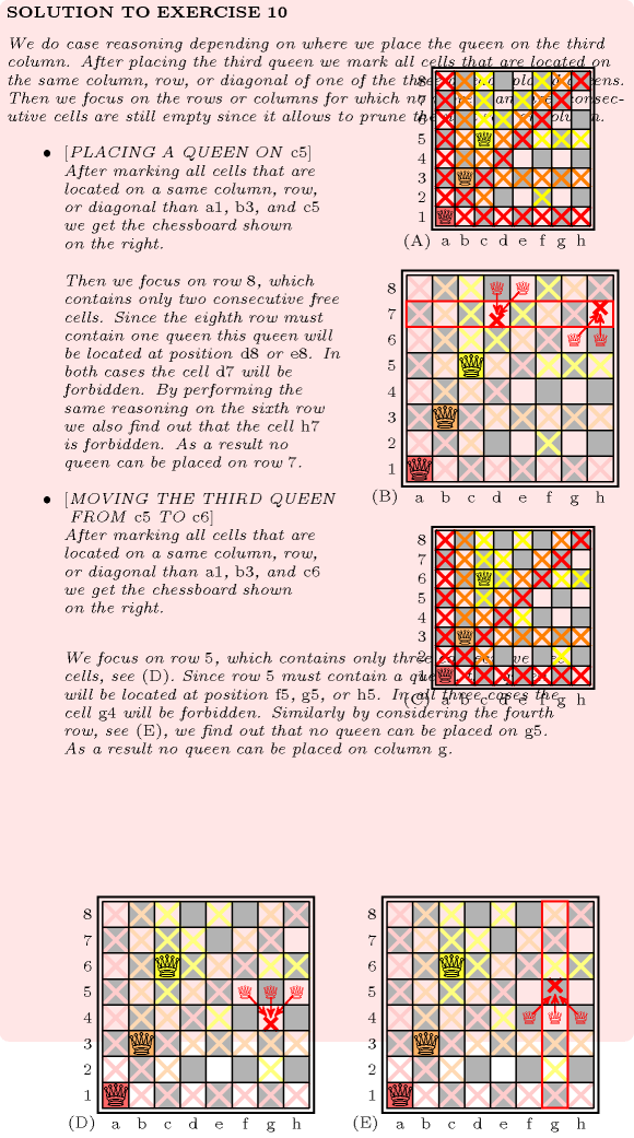
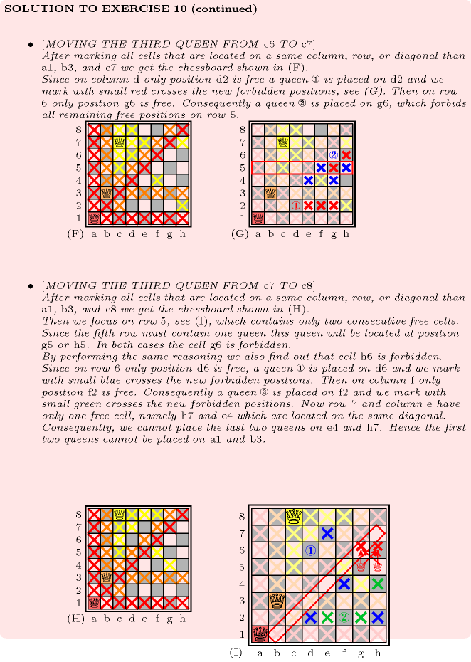
: (8-queens) unfeasibility of a partial solution