5.137. elem
| DESCRIPTION | LINKS | GRAPH | AUTOMATON |
- Origin
- Constraint
- Usual name
- Synonyms
, .
- Arguments
- Restrictions
- Purpose
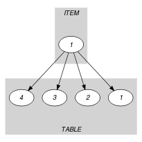
is equal to one of the entries of the table .
- Example
-
The constraint holds since its first argument corresponds to the third item of the collection.
- Typical
- Symmetries
Items of are permutable.
All occurrences of two distinct values in or can be swapped; all occurrences of a value in or can be renamed to any unused value.
- Arg. properties
Functional dependency: determined by and .
- Usage
Makes the link between the discrete decision variable and the variable according to a given table of values . We now give five typical uses of the constraint.
In some problems we may have to represent a function (with ). In this context we generate the following constraint where is a domain variable taking its values in :
Figure 5.137.1. ()
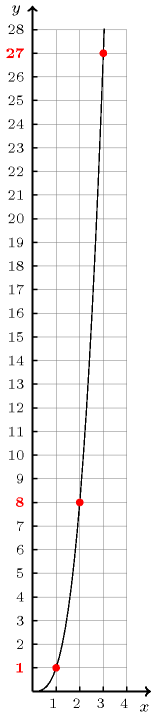
As an example, consider the problem of finding the smallest integer that can be decomposed in two different ways in the sum of two cubes [HardyWright75]. The constraint can be used for representing the function (Figure 5.137.1). The unique solution can be obtained by the following set of constraints:
The last three inequalities constraints in the conjunction are used for breaking symmetries. The constraints and respectively order the pairs of variables and from which the sums and are generated. Finally the inequality enforces a lexicographic ordering between the two pairs of variables and .
In some optimisation problems a classical use of the constraint consists expressing the link between a discrete choice and its corresponding cost. For each discrete choice we create an constraint of the form:
where:
is a domain variable that indicates which alternative will be finally selected,
is a domain variable that corresponds to the cost of the decision associated with the value of the variable,
are the respective costs associated with the alternatives .
In some problems we need to express a disjunction of the form . This can be directly reformulated as the following constraint, where is a domain variable taking its value in the finite set and where the argument corresponds to the domain variables :
In some scheduling problems the duration of a task depends on the machine where the task will be assigned in final schedule. In this case we generate for each task an constraint of the following form:
where:
is a domain variable that indicates the resource to which the task will be assigned,
is a domain variable that corresponds to the duration of the task,
are the respective duration of the task according to the hypothesis that it runs on machine or .
Figure 5.137.2. A task for which the duration depends on the machine 1, 2 or 3 to which it is assigned
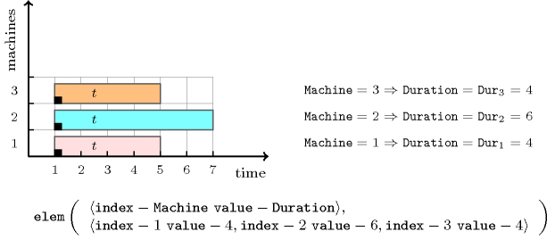
Figure 5.137.2 illustrates this particular use of the constraint for modelling that a task has a duration of 4, 6 and 4 when we respectively assign it on machines 1, 2 and 3.
In some vehicle routing problems we typically use the constraint to express the distance between location and the next location visited by a vehicle. For this purpose we generate for each location an constraint of the form:
where:
is a domain variable that gives the index of the location the vehicle will visit just after location ,
is a domain variable that corresponds to the distance between location and the location the vehicle will visit just after,
are the respective distances between location and locations .
An other example where the table argument corresponds to domain variables is described in the keyword entry assignment to the same set of values.
- Remark
Originally, the parameters of the constraint had the form , where and were two domain variables and was a list of non-negative integers.
Within some systems (e.g., Gecode), the index of the first entry of the table corresponds to 0 rather than to 1.
When the first entry of the table corresponds to a value that is different from 1 we can still use the constraint. We use the reformulation , where and are domain variables respectively ranging from 1 to and from to .
- Systems
nth in Choco, element in Gecode, element in JaCoP, element in SICStus.
- See also
common keyword: , , , (array constraint), , (data constraint).
implies: (single item replaced by two variables), , , .
- Keywords
characteristic of a constraint: automaton, automaton without counters, reified automaton constraint.
constraint arguments: pure functional dependency.
constraint network structure: centered cyclic(2) constraint network(1).
constraint type: data constraint.
heuristics: labelling by increasing cost, regret based heuristics.
modelling: array constraint, table, functional dependency, variable indexing, variable subscript, disjunction, assignment to the same set of values, sequence dependent set-up.
modelling exercises: assignment to the same set of values, sequence dependent set-up, zebra puzzle.
- Cond. implications
- Arc input(s)
- Arc generator
-
- Arc arity
- Arc constraint(s)
-
- Graph property(ies)
-
- Graph model
We regroup the and parameters of the original constraint into the parameter . We also make explicit the different indices of the table .
Parts (A) and (B) of Figure 5.137.3 respectively show the initial and final graph associated with the Example slot. Since we use the graph property, the unique arc of the final graph is stressed in bold.
Figure 5.137.3. Initial and final graph of the constraint

(a) (b) - Signature
Since all the attributes of are distinct and because of the first condition of the arc constraint the final graph cannot have more than one arc. Therefore we can rewrite to and simplify to .
- Automaton
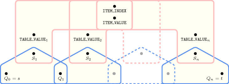
Figure 5.137.4 depicts the automaton associated with the constraint. Let and respectively be the and the attributes of the unique item of the collection. Let and respectively be the and the attributes of item of the collection. To each quadruple corresponds a 0-1 signature variable as well as the following signature constraint: .
Figure 5.137.4. Automaton of the constraint (once one finds the right item – index and value – in the table, one switches from the initial state to the accepting state )
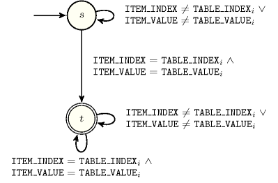
Figure 5.137.5. Hypergraph of the reformulation corresponding to the automaton of the constraint