Global Constraint Catalog: Cminimum_weight

5.266. minimum_weight_alldifferent

DESCRIPTION

LINKS

GRAPH

Origin

[FocacciLodiMilano99]

Constraint

$𝚖𝚒𝚗𝚒𝚖𝚞𝚖_𝚠𝚎𝚒𝚐𝚑𝚝_𝚊𝚕𝚕𝚍𝚒𝚏𝚏𝚎𝚛𝚎𝚗𝚝 (𝚅𝙰𝚁𝙸𝙰𝙱𝙻𝙴𝚂, 𝙼𝙰𝚃𝚁𝙸𝚇, 𝙲𝙾𝚂𝚃)$

Synonyms

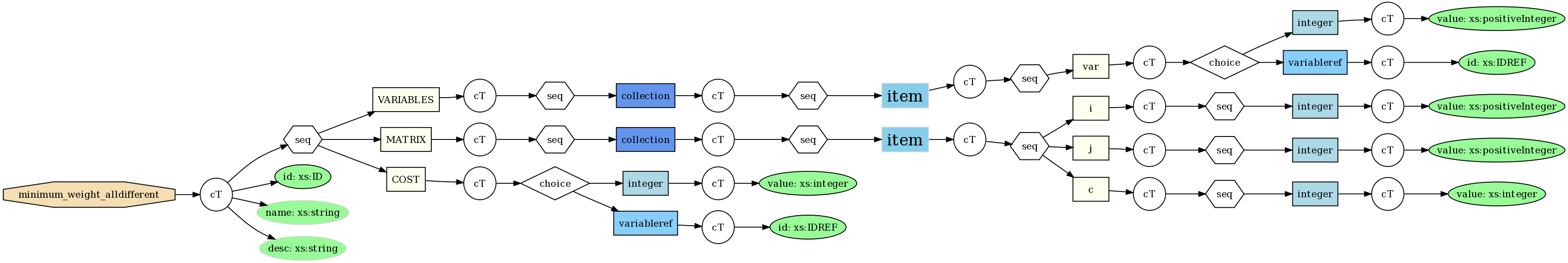
$𝚖𝚒𝚗𝚒𝚖𝚞𝚖_𝚠𝚎𝚒𝚐𝚑𝚝_𝚊𝚕𝚕𝚍𝚒𝚏𝚏$ , $𝚖𝚒𝚗𝚒𝚖𝚞𝚖_𝚠𝚎𝚒𝚐𝚑𝚝_𝚊𝚕𝚕𝚍𝚒𝚜𝚝𝚒𝚗𝚌𝚝$ , $𝚖𝚒𝚗_𝚠𝚎𝚒𝚐𝚑𝚝_𝚊𝚕𝚕𝚍𝚒𝚏𝚏$ , $𝚖𝚒𝚗_𝚠𝚎𝚒𝚐𝚑𝚝_𝚊𝚕𝚕𝚍𝚒𝚏𝚏𝚎𝚛𝚎𝚗𝚝$ , $𝚖𝚒𝚗_𝚠𝚎𝚒𝚐𝚑𝚝_𝚊𝚕𝚕𝚍𝚒𝚜𝚝𝚒𝚗𝚌𝚝$ .

Arguments

$𝚅𝙰𝚁𝙸𝙰𝙱𝙻𝙴𝚂$	$𝚌𝚘𝚕𝚕𝚎𝚌𝚝𝚒𝚘𝚗 (𝚟𝚊𝚛 - 𝚍𝚟𝚊𝚛)$
$𝙼𝙰𝚃𝚁𝙸𝚇$	$𝚌𝚘𝚕𝚕𝚎𝚌𝚝𝚒𝚘𝚗 (𝚒 - 𝚒𝚗𝚝, 𝚓 - 𝚒𝚗𝚝, 𝚌 - 𝚒𝚗𝚝)$
$𝙲𝙾𝚂𝚃$	$𝚍𝚟𝚊𝚛$

Restrictions

| 𝚅𝙰𝚁𝙸𝙰𝙱𝙻𝙴𝚂 | > 0

𝚛𝚎𝚚𝚞𝚒𝚛𝚎𝚍

(𝚅𝙰𝚁𝙸𝙰𝙱𝙻𝙴𝚂, 𝚟𝚊𝚛)

𝚅𝙰𝚁𝙸𝙰𝙱𝙻𝙴𝚂 . 𝚟𝚊𝚛 \geq 1

𝚅𝙰𝚁𝙸𝙰𝙱𝙻𝙴𝚂 . 𝚟𝚊𝚛 \leq | 𝚅𝙰𝚁𝙸𝙰𝙱𝙻𝙴𝚂 |

𝚛𝚎𝚚𝚞𝚒𝚛𝚎𝚍

(𝙼𝙰𝚃𝚁𝙸𝚇, [𝚒, 𝚓, 𝚌])

𝚒𝚗𝚌𝚛𝚎𝚊𝚜𝚒𝚗𝚐_𝚜𝚎𝚚

(𝙼𝙰𝚃𝚁𝙸𝚇, [𝚒, 𝚓])

𝙼𝙰𝚃𝚁𝙸𝚇 . 𝚒 \geq 1

𝙼𝙰𝚃𝚁𝙸𝚇 . 𝚒 \leq | 𝚅𝙰𝚁𝙸𝙰𝙱𝙻𝙴𝚂 |

𝙼𝙰𝚃𝚁𝙸𝚇 . 𝚓 \geq 1

𝙼𝙰𝚃𝚁𝙸𝚇 . 𝚓 \leq | 𝚅𝙰𝚁𝙸𝙰𝙱𝙻𝙴𝚂 |

| 𝙼𝙰𝚃𝚁𝙸𝚇 | = | 𝚅𝙰𝚁𝙸𝙰𝙱𝙻𝙴𝚂 | * | 𝚅𝙰𝚁𝙸𝙰𝙱𝙻𝙴𝚂 |

Purpose

All variables of the $𝚅𝙰𝚁𝙸𝙰𝙱𝙻𝙴𝚂$ collection should take a distinct value located within interval $[1, | 𝚅𝙰𝚁𝙸𝙰𝙱𝙻𝙴𝚂 |]$ . In addition $𝙲𝙾𝚂𝚃$ is equal to the sum of the costs associated with the fact that we assign value $i$ to variable $j$ . These costs are given by the matrix $𝙼𝙰𝚃𝚁𝙸𝚇$ .

Example

(\begin{matrix} 〈2, 3, 1, 4〉, \\ 〈\begin{matrix} 𝚒 - 1 & 𝚓 - 1 & 𝚌 - 4, \\ 𝚒 - 1 & 𝚓 - 2 & 𝚌 - 1, \\ 𝚒 - 1 & 𝚓 - 3 & 𝚌 - 7, \\ 𝚒 - 1 & 𝚓 - 4 & 𝚌 - 0, \\ 𝚒 - 2 & 𝚓 - 1 & 𝚌 - 1, \\ 𝚒 - 2 & 𝚓 - 2 & 𝚌 - 0, \\ 𝚒 - 2 & 𝚓 - 3 & 𝚌 - 8, \\ 𝚒 - 2 & 𝚓 - 4 & 𝚌 - 2, \\ 𝚒 - 3 & 𝚓 - 1 & 𝚌 - 3, \\ 𝚒 - 3 & 𝚓 - 2 & 𝚌 - 2, \\ 𝚒 - 3 & 𝚓 - 3 & 𝚌 - 1, \\ 𝚒 - 3 & 𝚓 - 4 & 𝚌 - 6, \\ 𝚒 - 4 & 𝚓 - 1 & 𝚌 - 0, \\ 𝚒 - 4 & 𝚓 - 2 & 𝚌 - 0, \\ 𝚒 - 4 & 𝚓 - 3 & 𝚌 - 6, \\ 𝚒 - 4 & 𝚓 - 4 & 𝚌 - 5 \end{matrix}〉, 17 \end{matrix})

The $𝚖𝚒𝚗𝚒𝚖𝚞𝚖_𝚠𝚎𝚒𝚐𝚑𝚝_𝚊𝚕𝚕𝚍𝚒𝚏𝚏𝚎𝚛𝚎𝚗𝚝$ constraint holds since the cost 17 corresponds to the sum $𝙼𝙰𝚃𝚁𝙸𝚇 [(1 - 1) \cdot 4 + 2] . 𝚌 + 𝙼𝙰𝚃𝚁𝙸𝚇 [(2 - 1) \cdot 4 + 3] . 𝚌 + 𝙼𝙰𝚃𝚁𝙸𝚇 [(3 - 1) \cdot 4 + 1] . 𝚌 + 𝙼𝙰𝚃𝚁𝙸𝚇 [(4 - 1) \cdot 4 + 4] . 𝚌 = 𝙼𝙰𝚃𝚁𝙸𝚇 [2] . 𝚌 + 𝙼𝙰𝚃𝚁𝙸𝚇 [7] . 𝚌 + 𝙼𝙰𝚃𝚁𝙸𝚇 [9] . 𝚌 + 𝙼𝙰𝚃𝚁𝙸𝚇 [16] . 𝚌 = 1 + 8 + 3 + 5$ .

All solutions

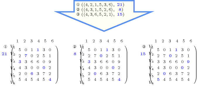
Figure 5.266.1 gives all solutions to the following non ground instance of the $𝚖𝚒𝚗𝚒𝚖𝚞𝚖_𝚠𝚎𝚒𝚐𝚑𝚝_𝚊𝚕𝚕𝚍𝚒𝚏𝚏𝚎𝚛𝚎𝚗𝚝$ constraint:

$V_{1} \in [2, 4]$ , $V_{2} \in [2, 3]$ , $V_{3} \in [1, 6]$ , $V_{4} \in [2, 5]$ , $V_{5} \in [2, 3]$ , $V_{6} \in [1, 6]$ , $C \in [0, 25]$ ,

$𝚖𝚒𝚗𝚒𝚖𝚞𝚖_𝚠𝚎𝚒𝚐𝚑𝚝_𝚊𝚕𝚕𝚍𝚒𝚏𝚏𝚎𝚛𝚎𝚗𝚝$ $(〈 V_{1}, V_{2}, V_{3}, V_{4}, V_{5}, V_{6} 〉$ ,

$〈 115, 120, 131, 141, 153, 160$ ,

$212, 227, 230, 242, 255, 261$ ,

$313, 323, 336, 346, 350, 369$ ,

$414, 423, 430, 440, 450, 462$ ,

$512, 520, 536, 543, 557, 562$ ,

$615, 624, 635, 644, 655, 664 〉, C)$ .

Figure 5.266.1. All solutions corresponding to the non ground example of the $𝚖𝚒𝚗𝚒𝚖𝚞𝚖_𝚠𝚎𝚒𝚐𝚑𝚝_𝚊𝚕𝚕𝚍𝚒𝚏𝚏𝚎𝚛𝚎𝚗𝚝$ constraint of the All solutions slot

Typical

| 𝚅𝙰𝚁𝙸𝙰𝙱𝙻𝙴𝚂 | > 1

𝚛𝚊𝚗𝚐𝚎

(𝙼𝙰𝚃𝚁𝙸𝚇 . 𝚌) > 1

𝙼𝙰𝚃𝚁𝙸𝚇 . 𝚌 > 0

Arg. properties

Functional dependency: $𝙲𝙾𝚂𝚃$ determined by $𝚅𝙰𝚁𝙸𝙰𝙱𝙻𝙴𝚂$ and $𝙼𝙰𝚃𝚁𝙸𝚇$ .

Algorithm

The Hungarian method for the assignment problem [Kuhn55] can be used for evaluating the bounds of the $𝙲𝙾𝚂𝚃$ variable. A filtering algorithm is described in [Sellmann02]. It can be used for handling both side of the $𝚖𝚒𝚗𝚒𝚖𝚞𝚖_𝚠𝚎𝚒𝚐𝚑𝚝_𝚊𝚕𝚕𝚍𝚒𝚏𝚏𝚎𝚛𝚎𝚗𝚝$ constraint:

Evaluating a lower bound of the $𝙲𝙾𝚂𝚃$ variable and pruning the variables of the $𝚅𝙰𝚁𝙸𝙰𝙱𝙻𝙴𝚂$ collection in order to not exceed the maximum value of $𝙲𝙾𝚂𝚃$ .
Evaluating an upper bound of the $𝙲𝙾𝚂𝚃$ variable and pruning the variables of the $𝚅𝙰𝚁𝙸𝙰𝙱𝙻𝙴𝚂$ collection in order to not be under the minimum value of $𝙲𝙾𝚂𝚃$ .

Systems

all_different in SICStus, all_distinct in SICStus.

common keyword: $𝚐𝚕𝚘𝚋𝚊𝚕_𝚌𝚊𝚛𝚍𝚒𝚗𝚊𝚕𝚒𝚝𝚢_𝚠𝚒𝚝𝚑_𝚌𝚘𝚜𝚝𝚜$ (cost filtering constraint,weighted assignment), $𝚜𝚞𝚖_𝚘𝚏_𝚠𝚎𝚒𝚐𝚑𝚝𝚜_𝚘𝚏_𝚍𝚒𝚜𝚝𝚒𝚗𝚌𝚝_𝚟𝚊𝚕𝚞𝚎𝚜$ (weighted assignment), $𝚠𝚎𝚒𝚐𝚑𝚝𝚎𝚍_𝚙𝚊𝚛𝚝𝚒𝚊𝚕_𝚊𝚕𝚕𝚍𝚒𝚏𝚏$ (cost filtering constraint,weighted assignment).

Keywords

application area: assignment.

characteristic of a constraint: core.

filtering: cost filtering constraint, Hungarian method for the assignment problem.

final graph structure: one_succ.

modelling: cost matrix, functional dependency.

problems: weighted assignment.

Arc input(s)

$𝚅𝙰𝚁𝙸𝙰𝙱𝙻𝙴𝚂$

Arc generator

𝐶𝐿𝐼𝑄𝑈𝐸

\mapsto 𝚌𝚘𝚕𝚕𝚎𝚌𝚝𝚒𝚘𝚗 (𝚟𝚊𝚛𝚒𝚊𝚋𝚕𝚎𝚜 1, 𝚟𝚊𝚛𝚒𝚊𝚋𝚕𝚎𝚜 2)

Arc arity

Arc constraint(s)

𝚟𝚊𝚛𝚒𝚊𝚋𝚕𝚎𝚜 1 . 𝚟𝚊𝚛 = 𝚟𝚊𝚛𝚒𝚊𝚋𝚕𝚎𝚜 2 . 𝚔𝚎𝚢

Graph property(ies)

•

𝐍𝐓𝐑𝐄𝐄

= 0

• 𝐒𝐔𝐌_𝐖𝐄𝐈𝐆𝐇𝐓_𝐀𝐑𝐂 (\begin{matrix} 𝙼𝙰𝚃𝚁𝙸𝚇 [\sum (\begin{matrix} (𝚟𝚊𝚛𝚒𝚊𝚋𝚕𝚎𝚜 1 . 𝚔𝚎𝚢 - 1) * | 𝚅𝙰𝚁𝙸𝙰𝙱𝙻𝙴𝚂 |, \\ 𝚟𝚊𝚛𝚒𝚊𝚋𝚕𝚎𝚜 1 . 𝚟𝚊𝚛 \end{matrix})] . 𝚌 \end{matrix}) = 𝙲𝙾𝚂𝚃

Graph model

Since each variable takes one value, and because of the arc constraint $𝚟𝚊𝚛𝚒𝚊𝚋𝚕𝚎𝚜 1 = 𝚟𝚊𝚛𝚒𝚊𝚋𝚕𝚎𝚜 . 𝚔𝚎𝚢$ , each vertex of the initial graph belongs to the final graph and has exactly one successor. Therefore the sum of the out-degrees of the vertices of the final graph is equal to the number of vertices of the final graph. Since the sum of the in-degrees is equal to the sum of the out-degrees, it is also equal to the number of vertices of the final graph. Since $𝐍𝐓𝐑𝐄𝐄 = 0$ , each vertex of the final graph belongs to a circuit. Therefore each vertex of the final graph has at least one predecessor. Since we saw that the sum of the in-degrees is equal to the number of vertices of the final graph, each vertex of the final graph has exactly one predecessor. We conclude that the final graph consists of a set of vertex-disjoint elementary circuits.

Finally the graph constraint expresses that the $𝙲𝙾𝚂𝚃$ variable is equal to the sum of the elementary costs associated with each variable-value assignment. All these elementary costs are recorded in the $𝙼𝙰𝚃𝚁𝙸𝚇$ collection. More precisely, the cost $c_{i j}$ is recorded in the attribute $𝚌$ of the ${((i - 1) \cdot | 𝚅𝙰𝚁𝙸𝙰𝙱𝙻𝙴𝚂) | + j)}^{t h}$ entry of the $𝙼𝙰𝚃𝚁𝙸𝚇$ collection. This is ensured by the $𝚒𝚗𝚌𝚛𝚎𝚊𝚜𝚒𝚗𝚐$ restriction that enforces that the items of the $𝙼𝙰𝚃𝚁𝙸𝚇$ collection are sorted in lexicographically increasing order according to attributes $𝚒$ and $𝚓$ .

Figure 5.266.2. Initial and final graph of the $𝚖𝚒𝚗𝚒𝚖𝚞𝚖_𝚠𝚎𝚒𝚐𝚑𝚝_𝚊𝚕𝚕𝚍𝚒𝚏𝚏𝚎𝚛𝚎𝚗𝚝$ constraint


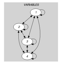
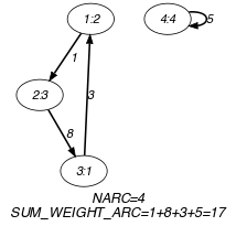
(a)	(b)

Parts (A) and (B) of Figure 5.266.2 respectively show the initial and final graph associated with the Example slot. Since we use the $𝐒𝐔𝐌_𝐖𝐄𝐈𝐆𝐇𝐓_𝐀𝐑𝐂$ graph property, the arcs of the final graph are stressed in bold. We also indicate their corresponding weight.

Global Constraint Catalog

5. Global Constraint Catalogue

5.266. minimum_weight_alldifferent

Figure 5.266.1. All solutions corresponding to the non ground example of the 𝚖𝚒𝚗𝚒𝚖𝚞𝚖_𝚠𝚎𝚒𝚐𝚑𝚝_𝚊𝚕𝚕𝚍𝚒𝚏𝚏𝚎𝚛𝚎𝚗𝚝 constraint of the All solutions slot

Figure 5.266.2. Initial and final graph of the 𝚖𝚒𝚗𝚒𝚖𝚞𝚖_𝚠𝚎𝚒𝚐𝚑𝚝_𝚊𝚕𝚕𝚍𝚒𝚏𝚏𝚎𝚛𝚎𝚗𝚝 constraint

Figure 5.266.1. All solutions corresponding to the non ground example of the $𝚖𝚒𝚗𝚒𝚖𝚞𝚖_𝚠𝚎𝚒𝚐𝚑𝚝_𝚊𝚕𝚕𝚍𝚒𝚏𝚏𝚎𝚛𝚎𝚗𝚝$ constraint of the All solutions slot

Figure 5.266.2. Initial and final graph of the $𝚖𝚒𝚗𝚒𝚖𝚞𝚖_𝚠𝚎𝚒𝚐𝚑𝚝_𝚊𝚕𝚕𝚍𝚒𝚏𝚏𝚎𝚛𝚎𝚗𝚝$ constraint