5.97. cumulative_convex
| DESCRIPTION | LINKS | GRAPH |
- Origin
- Constraint
- Type
- Arguments
- Restrictions
- Purpose
Cumulative scheduling constraint or scheduling under resource constraints. Consider a set of tasks described by the collection where each task is defined by:
A set of distinct points depicting the time interval where the task is actually running: the smallest and largest coordinates of these points respectively give the first and last instant of that time interval.
A height that depicts the resource consumption used by the task from its first instant to its last instant.
The constraint enforces that, at each point in time, the cumulated height of the set of tasks that overlap that point, does not exceed a given limit. A task overlaps a point if and only if (1) its origin is less than or equal to , and (2) its end is strictly greater than .
- Example
-
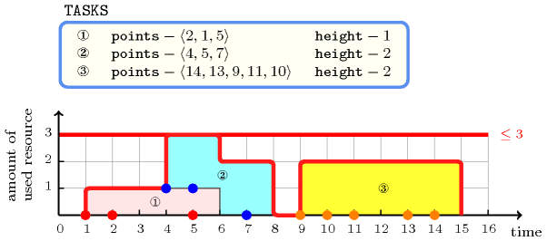
Figure 5.97.1 shows the cumulated profile associated with the example. To each set of points defining a task corresponds a rectangle. The height of each rectangle represents the resource consumption of the associated task. The constraint holds since at each point in time we do not have a cumulated resource consumption strictly greater than the upper limit 3 enforced by the last argument of the constraint.
Figure 5.97.1. Points defining the three tasks of the Example slot and corresponding resource consumption profile (note that the vertical position of a task does not really matter but is only used for displaying the contribution of a task to the resource consumption profile)

- Typical
- Symmetries
Items of are permutable.
Items of are permutable.
can be decreased to any value .
can be increased.
- Arg. properties
Contractible wrt. .
- Usage
A natural use of the constraint corresponds to problems where a task is defined as the convex hull of a set of distinct points that are not initially fixed. Note that, by explicitly introducing a start and an end variables, and by using a and a constraints, one could replace the constraint by a constraint. However this hinders propagation.
As a concrete example of use of the constraint we present a constraint model for a well-known pattern-sequencing problem [FinkVoss99] (also known to be equivalent to the graph path-width [LinharesYanasse02] problem) that is based on a single constraint. The pattern sequencing problem can be described as follows: Given a 0-1 matrix in which each column corresponds to a product required by the customers and each row corresponds to the order of a particular customer (The entry is equal to 1 if and only if customer has ordered some quantity of product .), the objective is to find a permutation of the products such that the maximum number of open orders at any point in the sequence is minimised. Order is open at point in the production sequence if there is a product required in order that appears at or before position in the sequence and also a product that appears at or after position in the sequence.
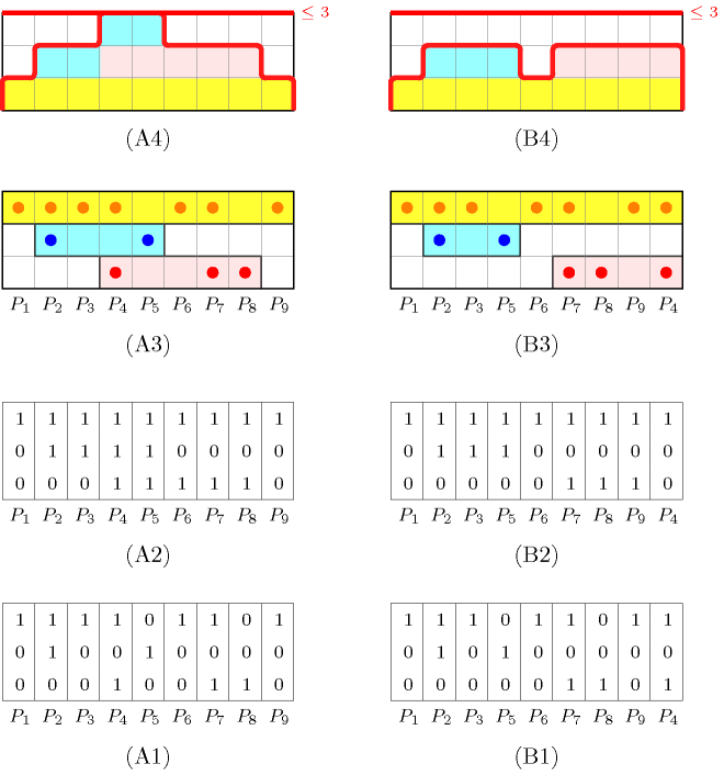
Figure 5.97.2. An input matrix for the pattern sequencing problem (A1), its corresponding cumulated matrix (A2), a view in term of tasks (A3) and the corresponding cumulative profile (A4); a second matrix (B1) where column 4 of (A1) is put at the rightmost position.

Before giving the constraint model, let us first provide an instance of the pattern-sequencing problem. Consider the matrix depicted by part (A1) of Fig. 5.97.2. Part (A2) gives its corresponding cumulated matrix obtained by setting to 1 each 0 of that is both preceded and followed by a 1. Part (A3) depicts the corresponding solution in term of the constraint: to each row of the matrix corresponds a task defined as the convex hull of the different 1 located on that row. Finally part (A4) gives the cumulated profile associated with part (A3), namely the number of 1 in each column of . The cost 3 of this solution is equal to the maximum number of 1 in the columns of the cumulated matrix . As shown by parts (B1-B4), we can get a lower cost of 2 by pushing the fourth column to the rightmost position.
The idea of the model is to associate to each row (i.e., customer) of the cumulated matrix a stack task that starts at the first 1 on row and ends at the last 1 of row (i.e., the task corresponds to the convex hull of the different 1 located on row ). Then the cost of a solution is simply the maximum height on the corresponding cumulated profile.
For each column of the 0-1 matrix initially given there is a variable ranging from 1 to the number of columns . The value of gives the position of column in a solution. We put all the stack tasks in a constraint, telling that each stack task uses one unit of the resource during all it execution. Since we want to have the same model for different limits on the maximum number of open stacks, and since all variables have to be distinct, we have an extra dummy task characterised as the convex hull of . This extra dummy task has a height that has to be maximised. For the matrix depicted by (A1) of Fig. 5.97.2 we pass to the constraint the following collection of tasks:
- Algorithm
A first natural way to handle the constraint is to accumulate the compulsory part [Lahrichi82] of the different tasks in a profile and to prune according to this profile. We give the main ideas for computing the compulsory part of a task and for pruning a task according to the profile of compulsory parts.
Compulsory part of a task Given a task characterised as the convex hull of a set of distinct points the compulsory part of corresponds to the, possibly empty, interval where:
is the largest value such that, when all variables are greater than or equal to , all variables can still take distinct values.
is the smallest value such that, when all variables are less than or equal to , all variables can still take distinct values.
Pruning according to the profile of compulsory parts Given two instants and and a task characterised as the convex hull of a set of distinct points , assume that cannot overlap and since this would lead exceeding , the second argument of the constraint. Furthermore assume that, when all variables are both greater than and less than , all variables cannot take distinct values. Then all values of can be removed from variables .
- See also
- Keywords
characteristic of a constraint: convex.
constraint type: scheduling constraint, resource constraint, temporal constraint.
- Derived Collection
- Arc input(s)
- Arc generator
-
- Arc arity
- Arc constraint(s)
- Graph property(ies)
-
- Arc input(s)
- Arc generator
-
- Arc arity
- Arc constraint(s)
- Graph class
-
- Sets
-
- Constraint(s) on sets
- Graph model
The first graph constraint forces for each task that the set of points defining its time interval are all distinct. The second graph constraint makes sure for each time point , that the cumulated heights of the tasks that overlap does not exceed the limit of the resource.
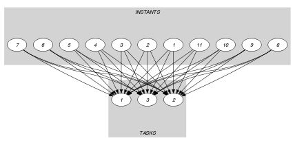
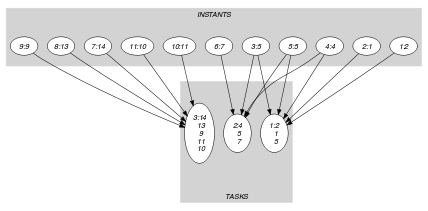
Parts (A) and (B) of Figure 5.97.3 respectively show the initial and final graph associated with the second graph constraint of the Example slot. On the one hand, each source vertex of the final graph can be interpreted as a time point corresponding to a point used in the definitions of the different tasks. On the other hand, the successors of a source vertex correspond to those tasks that overlap a given time point. The constraint holds since, for each successor set of the final graph, the sum of the heights of the tasks in does not exceed the limit .
Figure 5.97.3. Initial and final graph of the constraint

(a) 
(b)